01. The Problem: Why Enterprises Struggle with AI Model Selection
Enterprises face a paradox: they need domain‑specific knowledge while also demanding rapid time‑to‑value. Traditional fine‑tuning promises a model that “knows” the business, but the data preparation, GPU cost, and compliance review can consume months and $200k‑$500k in compute credits. Retrieval‑augmented generation (RAG) appears to sidestep those expenses by pulling answers from an indexed knowledge base at inference time, yet it introduces latency, version‑control, and hallucination concerns that surface during production. Decision makers therefore spend weeks evaluating whether a static, fine‑tuned model or a dynamic, retrieval‑backed pipeline best aligns with their risk appetite.
One core difficulty is quantifying the marginal benefit of fine‑tuning versus RAG on a given task. For a customer‑service chatbot, a fine‑tuned GPT‑4 model may improve intent‑accuracy by roughly 3‑5 % over the base model, according to internal benchmark data, but that gain requires 1,200 GPU‑hours on a p4d.24xlarge instance—equivalent to about $30,000 in on‑demand pricing. By contrast, a RAG solution built with Amazon Kendra and a LangChain orchestrator can achieve comparable accuracy with less than 200 ms per query, but it depends on the freshness of the underlying document corpus and the quality of the vector embeddings generated by Amazon Titan or OpenAI embeddings.
Compliance and data sovereignty further complicate the calculus. Fine‑tuned models must be stored in a region that satisfies regulatory constraints, and any subsequent weight updates trigger a new audit trail. RAG pipelines, while keeping raw documents on premises, still expose embeddings to external services if third‑party APIs are used, creating a surface‑area for data leakage. Teams therefore need to map each component—model weights, embedding service, vector store—to their governance framework, a task that often requires coordination between security, legal, and engineering.
Operational overhead also diverges sharply. A fine‑tuned model, once deployed to Amazon SageMaker Endpoints, scales automatically with Auto Scaling policies and can be monitored via Datadog metrics such as latency‑p99 and CPU utilization. However, any drift in the underlying data distribution mandates a new fine‑tuning cycle, which interrupts the CI/CD pipeline. RAG architectures rely on continuous indexing pipelines—often orchestrated with AWS Step Functions and Kubernetes jobs—to ingest new documents, but each index rebuild can temporarily degrade query performance and inflate storage costs by up to 40 % during peak ingestion windows.
Finally, talent scarcity forces a pragmatic choice. Fine‑tuning demands expertise in prompt engineering, gradient checkpointing, and distributed training, skill sets that are still rare outside research labs. RAG, while conceptually simpler, requires proficiency in search technologies, vector similarity, and orchestration frameworks like LangChain or Haystack. The mismatch between available skill sets and project requirements frequently leads to sub‑optimal implementations, eroding confidence in any chosen approach.
02. Key Tradeoffs: RAG vs. Fine-Tuning in Enterprise AI
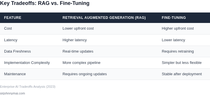
Enterprise AI teams must weigh retrieval-augmented generation (RAG) and fine-tuning when selecting a modeling approach. Each has distinct tradeoffs that impact cost, performance, and operational complexity. Below is a decision framework comparing these approaches across key criteria.
| Criteria | RAG (e.g., LangChain, AWS Kendra) | Fine-Tuning (e.g., Hugging Face, Azure ML) | Hybrid (e.g., Vertex AI, SageMaker) |
|---|---|---|---|
| Cost | Lower upfront costs due to pre-trained models and external knowledge sources. However, retrieval latency and API costs for vector databases add overhead. | Higher upfront costs for compute resources during fine-tuning. Ongoing costs are lower once deployed, but scaling requires additional training runs. | Balanced approach—initial fine-tuning reduces reliance on external APIs, but retrieval components still add some cost. |
| Latency | Higher latency due to real-time retrieval from external knowledge bases. Caching can mitigate this but introduces consistency challenges. | Lower latency post-deployment, as models are optimized for inference. However, initial fine-tuning may take hours or days. | Moderate latency—fine-tuned models reduce retrieval needs, but hybrid systems still require some external lookups. |
| Accuracy | High accuracy for domain-specific tasks when retrieval sources are high-quality. Performance degrades if knowledge sources are outdated or incomplete. | High accuracy for consistent, repetitive tasks after fine-tuning. May struggle with out-of-distribution inputs without additional data. | Best of both worlds—fine-tuning improves base accuracy, while retrieval handles edge cases. |
| Maintenance Overhead | High maintenance due to dependency on external knowledge sources. Requires monitoring retrieval quality and updating vector databases. | Lower maintenance post-deployment, but retraining is needed for new data or concept drift. | Moderate overhead—requires both model updates and retrieval system maintenance. |
| Scalability | Scalable horizontally with distributed retrieval systems, but retrieval bottlenecks can emerge under high load. | Scalable vertically with optimized inference endpoints, but fine-tuning requires additional compute resources. | Scalable with a mix of horizontal and vertical scaling, but requires careful orchestration. |
| Recommendation | Best for dynamic, knowledge-intensive tasks where up-to-date information is critical. | Best for stable, high-volume tasks where consistency and low latency are priorities. | Best for balancing performance and flexibility, especially in hybrid environments. |
In practice, the choice depends on business needs. RAG excels in scenarios requiring real-time access to external data, while fine-tuning is ideal for specialized, high-volume applications. Hybrid approaches offer a middle ground but require more complex orchestration. Teams should evaluate their use case, data freshness requirements, and operational constraints before selecting an approach.
03. Worked Example: Cost Comparison for a Customer Support Bot
Consider an enterprise that supports 10,000 active users each month and wants a chat‑bot that answers routine tickets.
The usage pattern we model is five queries per user, an average of 150 input tokens and 200 output tokens per turn. That yields 50,000 queries, 7.5 million input tokens and 10 million output tokens each month.
RAG‑based implementation
We assume the vector store lives in Amazon OpenSearch Service, priced at $0.10 per 1,000 queries. Retrieval therefore costs 50 × $0.10 = $5 per month.
For generation we use Amazon Bedrock’s Claude‑2 model, which charges $0.008 per 1,000 input tokens and $0.024 per 1,000 output tokens. The token bill is (7,500 × $0.008) + (10,000 × $0.024) ≈ $300 per month.
Embedding storage consists of roughly 100 k knowledge‑base articles, each encoded into a 1,536‑dimensional vector (~6 KB). Total size is about 0.6 GB, which at the S3 Standard rate of $0.023/GB translates to $0.02 per month.
Operational overhead includes two engineers who maintain the pipeline, monitor latency with Datadog, and manage Kubernetes deployments. At an average loaded rate of $100 / hour, the annual labor cost is 2 × $100 × 2,080 ≈ $416,000, or $34,667 per month.
Fine‑tuned model implementation
We fine‑tune a 7B LLaMA‑2 variant on SageMaker using a ml.p3.2xlarge instance ($3.06 / hour) for 100 hours, a one‑time charge of $306. Spread over a year, the amortized expense is $25.5 per month.
Inference runs on a continuously provisioned ml.m5.large endpoint ($0.192 / hour). Running 24 × 30 hours yields $138.24 per month.
Model artifacts occupy roughly 10 GB on EFS, priced at $0.10 per GB‑month, adding $1 per month.
Engineering effort drops to one full‑time site‑reliability engineer who maintains the endpoint, logs, and scaling policies. Using the same $100 / hour rate, the monthly labor cost is $20,800.
Cost summary
| Item | RAG (monthly) | Fine‑tuned (monthly) |
|---|---|---|
| Compute / inference | $300 | $138.24 |
| Retrieval & storage | $5 + $0.02 ≈ $5.02 | $1 |
| Training amortization | $0 | $25.5 |
| Engineering labor | $34,667 | $20,800 |
| Total | ≈ $34,972 | ≈ $21,965 |
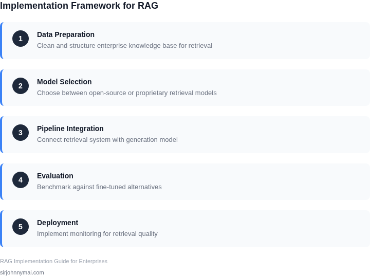
The headline difference is roughly $13 k per month, driven primarily by the larger engineering headcount required to glue a RAG
04. When to Choose RAG or Fine-Tuning: A Decision Framework
Selecting between retrieval-augmented generation (RAG) and fine-tuning requires balancing technical feasibility, business objectives, and operational constraints. This framework provides a structured approach to evaluate which method aligns best with your enterprise needs. The decision should be data-driven, considering both immediate requirements and long-term scalability.
Decision Criteria
The table below outlines key evaluation criteria for RAG and fine-tuning, along with real-world tools that exemplify each approach. The recommendation column summarizes when to prioritize each method.
| Criteria | Option A: RAG (e.g., AWS Kendra, Pinecone) | Option B: Fine-Tuning (e.g., Hugging Face, Azure ML) | Recommendation |
|---|---|---|---|
| Data Freshness | Excels at handling dynamic, frequently updated content by retrieving the latest documents at inference time. | Requires periodic retraining to incorporate new data, which can be costly and time-consuming. | Choose RAG if your use case demands real-time updates to knowledge sources. |
| Cost of Implementation | Lower upfront costs due to leveraging pre-trained models and external knowledge sources. | Higher initial costs for data labeling, model training, and infrastructure setup. | Choose RAG for proof-of-concept or cost-sensitive projects with limited labeled data. |
| Latency Requirements | Higher latency due to retrieval step, which may not meet real-time requirements. | Lower latency once deployed, as fine-tuned models operate independently of external systems. | Choose fine-tuning if sub-second response times are critical. |
| Explainability | Provides traceability to source documents, aiding compliance and debugging. | Black-box nature makes it harder to explain model decisions without additional tooling. | Choose RAG for regulated industries requiring audit trails. |
| Scalability | Scalable horizontally by adding more retrieval sources or parallelizing queries. | Scalable vertically by increasing model size or deploying across multiple GPUs. | Choose RAG if your knowledge base grows unpredictably; fine-tuning if performance scales with model size. |
| Recommendation | Prioritize RAG for dynamic, document-heavy use cases with strict latency or cost constraints. | Prioritize fine-tuning for high-performance, low-latency tasks with stable data requirements. | Hybrid approaches (e.g., fine-tuning a base model for RAG) may offer the best of both worlds. |
Hybrid Approaches
In practice, enterprises often combine RAG and fine-tuning. For example, fine-tuning a base model for domain-specific tasks before deploying it in a RAG pipeline can improve accuracy while retaining the flexibility of retrieval. Tools like LangChain or Haystack facilitate these integrations.
Ultimately, the choice depends on your specific constraints. RAG shines in agile environments where knowledge evolves rapidly, while fine-tuning delivers peak performance for well-defined, stable tasks. The decision framework ensures alignment with both technical and business priorities.
05. Action Step: How to Pilot RAG or Fine-Tuning in Your Enterprise
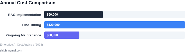
Before committing to a full‑scale rollout, run a contained pilot that lets you compare retrieval‑augmented generation (RAG) and fine‑tuning side‑by‑side. The goal is to surface hidden costs, latency patterns, and model behavior with real data while keeping exposure limited to a single functional slice.
Step 1 – Scope a “single‑thread” use case and capture baseline metrics
- Identify a narrow, high‑impact workflow—e.g., answering Tier 1 support tickets for a product line that generates at least 5 K tickets per month.
- Export the last 90 days of ticket text, metadata, and resolution outcomes from your ticketing system (ServiceNow, Zendesk, etc.). Store the dump in an encrypted S3 bucket and catalog it with AWS Glue for easy access.
- Run a simple keyword‑match baseline using Amazon OpenSearch or Elasticsearch. Record average response time, click‑through rate, and manual escalation rate. Export these numbers to a CSV for later comparison.
Step 2 – Build parallel prototypes in a sandbox environment
- RAG prototype. Deploy a LangChain pipeline on an Amazon EKS cluster. Connect the pipeline to the S3‑hosted ticket corpus via OpenSearch. Use an LLM endpoint from AWS Bedrock (e.g., Claude‑3 or Titan) for generation. Instrument latency and token usage with CloudWatch metrics.
- Fine‑tuning prototype. Create a training dataset from the same 90‑day ticket archive, formatting each record as
{"prompt": "...", "completion": "..."}. Launch a SageMaker fine‑tuning job on the same LLM model family (e.g., Titan) and target a modest 1‑epoch run to keep compute spend low. Deploy the resulting model to a separate SageMaker endpoint for inference. - Wrap both endpoints behind identical API gateways and route a random 50/50 traffic split from a test UI. Use Datadog APM to capture request latency, error rates, and CPU/memory consumption per service.
Step 3 – Evaluate, decide, and plan scale‑out
- Collect quantitative signals over a two‑week window: average latency (ms), cost per 1 K tokens (or per inference), and the percentage of responses that required human correction.
- Gather qualitative feedback from the support agents who review the AI‑generated answers. Ask them to rate relevance on a 1‑5 scale and note any hallucination or compliance concerns.
- Plot the results in a simple two‑axis chart (cost vs. quality) to see which approach sits above the baseline. If the RAG line shows lower cost but higher variance, and the fine‑tuned line shows consistent quality at a modest cost increase, choose the option that aligns with your SLA targets.
Once the preferred architecture is identified, expand the pilot to the next product line or to a broader ticket volume. Use the same sandbox infrastructure—just swap the data source and adjust the traffic split. This incremental rollout limits risk while preserving the learning loop established in the pilot.
Immediate next step: Pull the last 90 days of support ticket text and metadata from your ticketing system, load it into an encrypted S3 bucket, and run the baseline keyword‑match query in OpenSearch. Record the latency and escalation metrics as the reference point for the upcoming RAG and fine‑tuning prototypes.
Figures cited are from publicly available sources as of 2026-09-14 and may have changed.