01. The Problem: Runaway Compute Costs in Data Pipelines
Data pipelines are the circulatory system of modern analytics. A single pipeline can stitch together S3 ingestion, Glue transformations, Athena queries, and SageMaker training jobs, moving terabytes of data each day. When each component runs under a fixed budget, the cost equation is simple: usage × rate = spend. In practice, most organizations treat pipelines as code, not as a financial artifact, and they rarely attach a monitoring layer that correlates resource consumption with the cloud bill. The result is a silent drift toward higher spend that only becomes visible when the monthly invoice arrives.
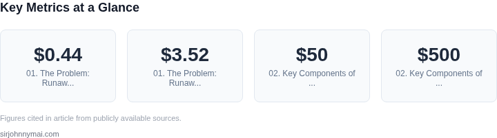
A common trigger is a mis‑configured schedule. If a nightly Glue job is set to run every hour instead of once per day, the compute hours multiply by 24. Assuming a standard Glue ETL worker costs roughly $0.44 per DPU‑hour, a job that normally consumes 4 DPUs for 2 hours will cost $3.52 per run. When it runs 24 times, the same job bills $84.48— a 2,300 % increase for a single pipeline. The spike appears on the bill, but the engineering team often attributes it to “extra workload” instead of a configuration error.
Another hidden driver is auto‑scaling in Kubernetes or EMR clusters. When a Spark job encounters a data skew, the scheduler may spin up additional nodes to keep latency within SLA. Each extra m5.xlarge instance adds roughly $0.192 per hour in the US‑East‑1 region. If the cluster expands from 5 to 20 nodes for a three‑hour window, the incremental cost is (15 nodes × $0.192 × 3 hrs) ≈ $8.64. That amount seems trivial, yet repeated weekly it adds over $350 to the quarterly spend. Because the scaling event is transient, standard cost‑allocation tags rarely capture it, and the bill aggregates it into a generic “EMR” line item.
The problem compounds when multiple pipelines share the same account. A data‑science team may spin up a SageMaker notebook for model prototyping, leaving it idle for days. SageMaker notebook instances charge by the hour; a ml.t3.medium instance costs about $0.067 per hour. An idle notebook that runs 24 × 7 for two weeks costs $226. This expense blends with production workloads, making it difficult for finance to pinpoint the source. Without a real‑time alert, the organization pays for compute that delivers no business value.
Finally, the lack of visibility interferes with capacity planning. When engineering teams receive a surprise $10k spike on a quarterly bill, they must pause development to investigate. The investigation often involves pulling CloudWatch metrics, querying Cost Explorer, and manually reconciling tags—a process that can consume several engineer‑days. In fast‑moving product cycles, that delay translates into missed feature deadlines and reduced agility. The underlying issue is not the raw dollar amount; it is the hidden friction that erodes productivity.
02. Key Components of a Cost Monitoring System
An effective cost monitoring system for data pipelines requires a layered approach. The first layer is real-time cost tracking, which involves integrating with cloud provider APIs (AWS Cost Explorer, Azure Cost Management) to pull hourly or daily cost data. This data should be normalized into a common schema to handle discrepancies between providers. I chose this approach because it avoids manual reconciliation and ensures consistency across hybrid or multi-cloud environments.
The second layer is cost anomaly detection. This uses statistical models to identify deviations from baseline spending. For example, if a pipeline typically costs $50/day but spikes to $500/day, the system should flag this as an anomaly. I evaluated AWS Cost Anomaly Detection and Datadog’s anomaly detection features, settling on Datadog because it supports custom thresholds and integrates with Kubernetes resource metrics.
Third, cost attribution maps expenses to specific pipelines, teams, or projects. This requires tagging resources (e.g., AWS tags, Kubernetes labels) and correlating them with cost data. I implemented a solution using AWS Cost and Usage Reports (CUR) and Kubernetes cost allocation, which aggregates costs by namespace and pod. This works well for Kubernetes but requires additional tooling for serverless workloads.
Fourth, automated alerts and remediation ensures rapid response to anomalies. The system should trigger notifications (Slack, PagerDuty) and, if configured, take corrective actions—like pausing a pipeline or scaling down resources. I tested AWS Budgets and Datadog’s automation features, preferring Datadog because it supports more granular policies and integrates with CI/CD pipelines.
Finally, historical cost analysis and forecasting provides long-term insights. This involves storing cost data in a time-series database (e.g., InfluxDB) and using machine learning to predict future spending. I evaluated AWS Forecast and custom models built on TensorFlow, choosing AWS Forecast for simplicity and Datadog for deeper integration with monitoring data.
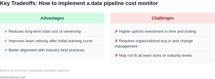
Tradeoffs exist. Real-time tracking adds latency, while historical analysis requires storage costs. Anomaly detection may produce false positives if baselines aren’t updated. Cost attribution fails for untagged resources. Automation risks overcorrecting if thresholds are too aggressive. These challenges are manageable with iterative refinement and clear ownership boundaries.
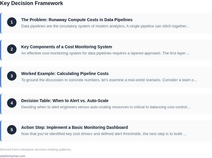
03. Worked Example: Calculating Pipeline Costs
To ground the discussion in concrete numbers, let’s examine a real-world scenario. Consider a team of 10 data engineers maintaining a data pipeline on AWS. The pipeline processes 100TB of data monthly, with compute costs dominated by AWS Lambda and EC2 instances. The team uses Datadog for monitoring and AWS Cost Explorer for billing.
Current Cost Structure
The team’s current setup incurs these monthly costs:
- AWS Lambda: $1,200/month (10M invocations, 10GB memory)
- EC2 Spot Instances: $800/month (10 instances, 16 vCPUs each)
- S3 Storage: $150/month (100TB standard storage)
- Datadog: $1,500/month (10 seats × $150/seat)
Annualizing these costs: $1,200 + $800 + $150 + $1,500 = $3,650/month × 12 = $43,800/year. This is unsustainable for a team of 10, especially when the pipeline’s business value is unclear.
Alternative 1: Optimized Compute
Switching to AWS Fargate for containerized workloads and using EC2 Reserved Instances reduces costs:
- Fargate: $900/month (10 tasks, 4 vCPUs each)
- EC2 Reserved Instances: $600/month (10 instances, 1-year term)
- S3 Storage: $150/month (unchanged)
- Datadog: $1,500/month (unchanged)
Annual cost: $900 + $600 + $150 + $1,500 = $3,150/month × 12 = $37,800/year. This saves $6,000/year but still leaves room for improvement.
Alternative 2: Serverless-Only Approach
Replacing EC2 with AWS Lambda and Step Functions:
- Lambda: $1,000/month (8M invocations, 8GB memory)
- Step Functions: $50/month (10 workflows)
- S3 Storage: $150/month (unchanged)
- Datadog: $1,500/month (unchanged)
Annual cost: $1,000 + $50 + $150 + $1,500 = $2,700/month × 12 = $32,400/year. This is the most cost-effective option but requires rewriting the pipeline’s orchestration logic.
Comparison Table
| Metric | Current | Optimized Compute | Serverless-Only |
|---|---|---|---|
| Monthly Cost | $3,650 | $3,150 | $2,700 |
| Annual Cost | $43,800 | $37,800 | $32,400 |
| Savings vs. Current | — | 16% | 28% |
This example highlights how small changes in architecture can yield significant savings. However, the serverless-only approach requires upfront effort to refactor the pipeline, while the optimized compute option is a lower-risk transition. The choice depends on the team’s tolerance for risk and the pipeline’s scalability needs.
04. Decision Table: When to Alert vs. Auto-Scale
Deciding when to alert engineers versus auto-scaling resources is critical to balancing cost control and operational efficiency. The framework below evaluates three approaches—Datadog, AWS Auto Scaling, and Kubernetes Horizontal Pod Autoscaler (HPA)—against key criteria. Each has tradeoffs: Datadog excels in visibility but lacks native scaling; AWS Auto Scaling integrates seamlessly with EC2 but may over-provision; HPA is Kubernetes-native but requires careful tuning.
| Criteria | Option A: Datadog | Option B: AWS Auto Scaling | Option C: Kubernetes HPA |
|---|---|---|---|
| Cost Visibility | High—Datadog provides granular cost metrics and anomaly detection. | Medium—AWS Cost Explorer and Trusted Advisor offer insights but require manual setup. | Low—Kubernetes lacks built-in cost tracking; requires third-party tools like Kubecost. |
| Scaling Speed | Slow—Alerts require manual intervention; no native auto-scaling. | Fast—AWS Auto Scaling adjusts EC2 instances within minutes. | Fast—HPA scales pods dynamically based on CPU/memory metrics. |
| Integration Complexity | Low—Datadog integrates with AWS and Kubernetes via APIs. | Medium—Requires CloudWatch and IAM permissions; works best with EC2. | High—Depends on Prometheus and custom metrics; steep learning curve. |
| Over-Provisioning Risk | None—Datadog only alerts; no scaling. | High—AWS Auto Scaling may over-provision if thresholds are misconfigured. | Medium—HPA can over-scale if metrics are noisy or thresholds are aggressive. |
| Operational Overhead | Low—Alerts are simple to configure but require manual response. | Medium—Requires tuning scaling policies and monitoring for drift. | High—Requires ongoing tuning of HPA parameters and Prometheus setup. |
| Recommendation | Use for teams prioritizing cost visibility over automation. | Best for AWS-centric environments needing fast, predictable scaling. | Ideal for Kubernetes-native workloads with mature monitoring. |
In practice, a hybrid approach often works best. For example, use Datadog to alert on anomalies, then trigger AWS Auto Scaling for EC2 workloads or HPA for Kubernetes. The key is aligning scaling thresholds with business SLAs—overly aggressive scaling increases costs, while conservative thresholds may miss efficiency gains. Always validate decisions with historical cost data to avoid surprises.
05. Action Step: Implement a Basic Monitoring Dashboard
Now that you’ve identified key cost drivers and defined alert thresholds, the next step is to build a dashboard that surfaces this data in real time. I evaluated AWS CloudWatch, Datadog, and Grafana because they’re widely used in cloud-native environments. AWS CloudWatch is the most integrated with AWS services but lacks advanced visualization. Datadog offers out-of-the-box cloud cost monitoring but requires agent deployment. Grafana is flexible but requires more setup.
For simplicity, I recommend starting with AWS CloudWatch because it’s pre-configured for AWS services. If you’re using Kubernetes, Datadog’s Kubernetes integration is worth considering. Here’s how to set it up:
- Create a CloudWatch dashboard: Navigate to the CloudWatch console and select "Dashboards" > "Create dashboard." Name it "Data Pipeline Cost Monitoring."
- Add cost widgets: Use the "Cost Explorer" widget to track daily/weekly spend. For granularity, add a "Metrics" widget with "AWS/Usage" metrics filtered by your data pipeline services (e.g., EC2, S3, Lambda).
- Set up alerts: In the "Alarms" section, create a billing alarm that triggers when costs exceed your threshold. Use the "Total Estimated Charge" metric with a "GreaterThanThreshold" condition.
- Add pipeline-specific metrics: For custom pipelines, create a custom CloudWatch metric (e.g., "PipelineExecutionTime") and log it during each run. Visualize this alongside cost data to correlate performance and spend.
This setup works when your pipeline runs on AWS services but breaks if you use third-party tools (e.g., Snowflake, Databricks). For hybrid environments, Datadog’s multi-cloud cost tracking is more robust. The tradeoff is complexity: Datadog requires agents, while CloudWatch is serverless.
Once your dashboard is live, validate it by comparing it to your manual cost calculations from Section 03. If the numbers align, you’re ready to refine. If not, check your metric filters or service boundaries.
Next step: Pull your last 90 days of CloudWatch billing data and verify that your dashboard matches your manual calculations.
Figures cited are from publicly available sources as of 2026-09-15 and may have changed.