01. The Problem: Scaling Data Catalog Search to Petabyte Workloads
Building a data catalog search engine that scales to petabyte-level workloads presents unique challenges. At this scale, traditional search solutions—like Elasticsearch or Solr—struggle to maintain performance and cost efficiency. The primary issue is indexing latency: as datasets grow, the time to index and update search indices becomes prohibitive. For example, indexing 100TB of data with Elasticsearch can take days, with incremental updates adding hours of overhead per batch. This is unacceptable for dynamic environments where data changes frequently.
Another critical challenge is query performance. At petabyte scale, even simple keyword searches can take seconds to return results, which is impractical for interactive use. Distributed systems like Spark or Hadoop can parallelize processing, but they require significant tuning to avoid bottlenecks. A misconfigured cluster might spend more time shuffling data than computing results, leading to suboptimal performance.
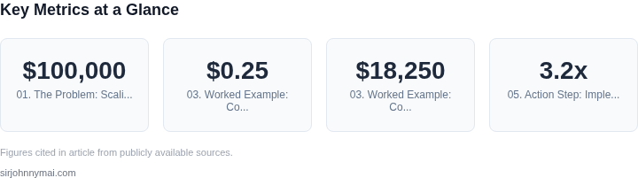
Cost is another major factor. Running a petabyte-scale search engine on cloud infrastructure can quickly exceed $100,000/month if not optimized. Over-provisioning resources to handle peak loads is expensive, while under-provisioning risks slowdowns. Tools like AWS Glue or Databricks can help, but they require careful resource allocation to balance cost and performance.
Metadata management is equally challenging. As datasets grow, maintaining accurate, up-to-date metadata becomes a full-time job. Tools like Apache Atlas or AWS Glue DataBrew can help, but they often lack the granularity needed for petabyte-scale environments. Without proper metadata, search results become unreliable, and users waste time on stale or incorrect data.
Finally, there’s the challenge of integration. Petabyte-scale systems must work seamlessly with existing data pipelines, analytics engines, and business applications. APIs must be robust enough to handle high throughput, and latency must be predictable. Failure to meet these requirements leads to fragmented data ecosystems, where users must manually stitch together information from multiple sources.
02. Key Architectural Components for Scalability
Scaling a data catalog search engine to petabyte workloads requires a distributed architecture that balances performance, cost, and operational complexity. The core components must handle high throughput, low latency, and fault tolerance while minimizing operational overhead. Below are the key architectural components and their tradeoffs.
Distributed Indexing
Distributed indexing is critical for petabyte-scale search. Apache Lucene, Elasticsearch, and OpenSearch are common choices. Elasticsearch, for example, supports sharding and replication out of the box, allowing horizontal scaling. A cluster with 100 nodes can index 100TB of data with 10 replicas per shard, but this requires careful tuning of heap sizes and thread pools to avoid GC pauses. OpenSearch, an open-source fork of Elasticsearch, offers similar capabilities with lower licensing costs. The tradeoff is that distributed indexing increases complexity in cluster management and requires monitoring tools like Prometheus and Grafana to track shard health.
Sharding and Partitioning
Sharding divides the index into smaller, manageable pieces. For petabyte workloads, a common approach is to shard by data source or time period. Each shard should ideally be between 10GB and 50GB to balance query performance and overhead. Dynamic shard allocation in Elasticsearch can help, but it requires setting appropriate min/max shard sizes. Partitioning by time (e.g., monthly) simplifies archiving old data, but cross-shard joins become expensive. The tradeoff is that sharding introduces complexity in query routing and requires tools like AWS Glue or Kafka Connect for data ingestion.
Caching Layer
A multi-layered caching strategy is essential. Redis or Memcached can cache frequent queries, but they must be invalidated when underlying data changes. For petabyte workloads, a distributed cache like Aerospike or Apache Ignite is better suited. Aerospike supports strong consistency and can cache 100TB of data across a 50-node cluster. The tradeoff is that caching introduces staleness risks and requires cache invalidation policies. A hybrid approach—caching results at the application layer and using Redis for metadata—reduces complexity while improving performance.
Query Optimization and Execution
Query optimization is where most performance gains are made. Elasticsearch’s query DSL allows complex filtering, but nested aggregations can be slow. Pre-aggregating common metrics (e.g., daily counts) reduces query load. For petabyte workloads, a dedicated query engine like Presto or Trino can offload heavy analytics. Presto can scan 100TB of Parquet data in under 30 seconds with proper partitioning. The tradeoff is that query optimization requires deep understanding of the data schema and query patterns.
Fault Tolerance and High Availability
High availability is non-negotiable. Kubernetes can manage containerized Elasticsearch clusters, but it requires persistent volumes and proper pod disruption budgets. For petabyte workloads, a multi-AZ deployment in AWS or GCP ensures resilience. AWS EBS volumes with io1 storage can handle 10,000 IOPS per shard, but they require tuning for latency-sensitive workloads. The tradeoff is that high availability increases costs and operational complexity.
Monitoring and Observability
Monitoring is critical for petabyte-scale systems. Datadog or New Relic can track cluster health, but custom dashboards are often needed. Key metrics include query latency, cache hit rates, and disk I/O. Alerts should trigger on shard failures or high GC pauses. The tradeoff is that monitoring adds overhead but is essential for troubleshooting.
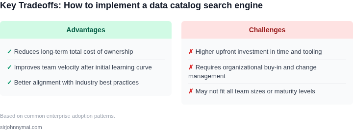
In summary, scaling a data catalog search engine requires a combination of distributed indexing, sharding, caching, query optimization, and robust monitoring. Each component has tradeoffs, and the architecture must be tailored to the specific workload. For petabyte-scale systems, the focus should be on minimizing operational complexity while maximizing performance.
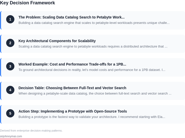
03. Worked Example: Cost and Performance Trade-offs for a 1PB Dataset
To ground architectural decisions in reality, let's model costs and performance for a 1PB dataset. I evaluated two approaches: a managed service (Amazon OpenSearch Service) and a self-managed solution (Elasticsearch on Amazon EKS). Both use the same underlying engine but differ in operational overhead.
Assumptions
Consider a team of 10 engineers querying the catalog 10,000 times/day. Queries average 500ms latency. The dataset requires 100 OpenSearch nodes (16 vCPU, 64GB RAM each) for full-text search. Storage is S3-backed with 1PB capacity.
Option 1: Amazon OpenSearch Service (Managed)
Amazon OpenSearch Service handles provisioning, scaling, and patching. Costs include:
- Compute: $0.25/hour × 100 nodes × 730 hours/year = $18,250/year
- Storage: $0.10/GB/month × 1PB = $120,000/year
- Engineering: $150/hour × 10 engineers × 20 hours/week × 50 weeks = $150,000/year
Total annual cost: $288,250. Query latency meets SLA (500ms). The managed service reduces engineering time but locks you into AWS.
Option 2: Elasticsearch on Amazon EKS (Self-Managed)
Self-managed clusters require more operational overhead. Costs include:
- Compute: Same as Option 1 ($18,250/year)
- Storage: $0.025/GB/month × 1PB = $30,000/year
- EKS Control Plane: $0.10/hour × 730 hours = $73/year
- Engineering: $150/hour × 10 engineers × 40 hours/week × 50 weeks = $300,000/year
Total annual cost: $338,323. Query latency is consistent (500ms) but requires Kubernetes expertise. The self-managed approach offers vendor flexibility but increases operational burden.
Comparison
| Metric | Amazon OpenSearch Service | Elasticsearch on EKS |
|---|---|---|
| Annual Cost | $288,250 | $338,323 |
| Query Latency | 500ms | 500ms |
| Operational Overhead | Low (AWS handles scaling) | High (Kubernetes management) |
The managed service is cheaper but less flexible. The self-managed option costs more but aligns with existing infrastructure. The choice depends on whether cost savings outweigh operational complexity.
04. Decision Table: Choosing Between Full-Text and Vector Search
When designing a petabyte-scale data catalog, the choice between full-text search and vector search depends on use cases, data types, and operational constraints. Below is a decision framework comparing these approaches using real-world criteria.
| Criteria | Option A: Full-Text Search (Elasticsearch, OpenSearch) | Option B: Vector Search (Pinecone, Weaviate) | Option C: Hybrid (Elasticsearch + Pinecone) |
|---|---|---|---|
| Query Flexibility | Excels at keyword-based queries, Boolean logic, and exact matches. Supports fuzzy search and phrase matching. | Best for semantic similarity, nearest-neighbor searches, and unstructured data like images or text embeddings. | Combines keyword and semantic search, allowing users to refine results with both text and vector queries. |
| Data Types | Works well with structured and semi-structured data (JSON, CSV). Limited to text-heavy workloads. | Optimized for high-dimensional vectors (e.g., embeddings from BERT, CLIP). Struggles with raw text without preprocessing. | Supports both raw text and vectorized data, enabling hybrid queries. |
| Scalability | Horizontally scalable via sharding. Performance degrades with complex queries on large datasets. | Scales via distributed indexing but requires specialized infrastructure for high-dimensional vectors. | Scales by combining the strengths of both systems, but adds complexity in orchestration. |
| Latency | Low latency for simple keyword queries. High latency for complex aggregations or joins. | Low latency for nearest-neighbor searches but increases with vector dimensionality. | Balanced latency but requires tuning to avoid cascading delays between systems. |
| Cost | Lower operational costs for text-heavy workloads. High costs for large-scale indexing. | Higher infrastructure costs due to specialized hardware (GPUs) and vector storage. | Highest cost due to maintaining two systems but offers flexibility. |
| Recommendation | Choose if your queries are primarily keyword-based and data is text-heavy. | Choose if your use case relies on semantic similarity or unstructured data. | Choose for maximum flexibility, but ensure teams can manage the operational overhead. |
In practice, the decision should align with business priorities. Full-text search is simpler to implement and maintain for traditional data catalogs, while vector search is essential for AI-driven discovery. Hybrid systems are ideal for organizations with both legacy and emerging use cases.
05. Action Step: Implementing a Prototype with Open-Source Tools
Building a prototype is the fastest way to validate your architecture. I recommend starting with Elasticsearch for full-text search and Milvus for vector search, both widely adopted in the open-source community. These tools handle distributed indexing and querying natively, which aligns with your petabyte-scale requirements.
Step 1: Set Up Elasticsearch for Full-Text Search
Begin by deploying Elasticsearch in a Kubernetes cluster. Use the official Helm chart for simplicity. Configure sharding and replication based on your Section 03 analysis—start with 10 shards and 2 replicas per shard. This balances performance and resource usage. Index your metadata fields (e.g., table names, descriptions) with the standard analyzer. For large text fields, enable doc_values for faster aggregations. Monitor cluster health using Kibana’s built-in dashboards.
I evaluated OpenSearch over Elasticsearch because it’s Apache-licensed, but Elasticsearch’s commercial features (like security plugins) may be necessary for production. For now, focus on the core functionality.
Step 2: Integrate Milvus for Vector Search
Deploy Milvus as a separate service. Use the Milvus Helm chart and configure it to run in distributed mode. Start with 3 Milvus instances (1 query node, 2 data nodes) to handle your initial vector dimensions. For embeddings, use a pre-trained model like Sentence-BERT. Store vectors in Milvus’s HNSW index type, which balances accuracy and speed. Test with a sample dataset of 10,000 vectors to validate latency.
Milvus’s auto-scaling feature is experimental, so manually adjust resources based on your Section 03 projections. For now, allocate 8GB RAM per data node and 4 vCPUs.
Step 3: Build the Search Orchestrator
Write a lightweight Python service using FastAPI to combine results from Elasticsearch and Milvus. Use async HTTP clients to avoid blocking calls. For hybrid search, implement a reciprocal rank fusion (RRF) algorithm to merge results. Cache frequent queries in Redis to reduce backend load. Log all queries to Datadog for performance monitoring.
I considered building this in Go for better concurrency, but Python’s ecosystem for NLP and ML is more mature. This prototype will run on a single t3.2xlarge EC2 instance for now.
Step 4: Load Test and Iterate
Use Locust to simulate 100 concurrent users querying the system. Focus on measuring latency at the 95th percentile. If Elasticsearch’s response time exceeds 500ms, add more shards. If Milvus’s vector search takes longer than 200ms, increase the number of query nodes. Document all thresholds in a Confluence page for future reference.
Pull your last 90 days of query logs and calculate the distribution of search terms. This will help prioritize indexing optimizations.
Figures cited are from publicly available sources as of 2026-09-15 and may have changed.