01. The Problem: Why Cold Starts Matter in Serverless
Serverless architectures promise scalability and cost efficiency by abstracting infrastructure management. However, cold starts—when a function is invoked after being idle—introduce unpredictable latency that can violate strict performance requirements. For example, a Lambda function might take 100ms to initialize, while a subsequent invocation could be as fast as 1-2ms. This inconsistency is unacceptable for applications like financial trading or real-time analytics, where latency must be consistently sub-10ms.
Cold starts occur because serverless platforms like AWS Lambda or Azure Functions provision resources on-demand. When a function hasn’t been used for a period (often minutes), the underlying container or VM must be reinitialized. This includes loading code, initializing runtime environments, and establishing network connections. The duration varies by platform: AWS Lambda typically experiences cold starts in the 50-500ms range, while Google Cloud Functions can take longer due to sandboxing overhead.
The impact isn’t just about speed. Cold starts can also strain downstream systems. A single cold start might trigger a cascade of dependent functions, each adding latency. For instance, a cold start in a microservices architecture could delay a user’s request by hundreds of milliseconds, leading to timeouts or degraded user experience. In high-throughput scenarios, this can result in cascading failures, as queues fill up and retries exacerbate the problem.
Cost considerations further complicate the tradeoff. While cold starts are free for AWS Lambda (you’re billed only for execution time), the latency penalty can be more expensive. A 500ms cold start might delay a response by 500ms, increasing the risk of user abandonment or compliance violations. For applications with strict SLAs, even occasional cold starts can trigger penalties or reputational damage.
Monitoring tools like Datadog or AWS CloudWatch can track cold starts, but they don’t solve the problem. Without proactive optimization, cold starts remain a hidden risk. The challenge is balancing cost savings with performance guarantees, especially when serverless is deployed in latency-sensitive domains like healthcare or autonomous systems.
02. Key Metrics and Evaluation Criteria
Evaluating cold start optimization requires measurable metrics that align with business requirements. For latency-sensitive applications, p99 latency is critical—it measures the worst-case 1% of requests. A well-optimized function should achieve p99 latencies within 100-200ms for interactive workloads, or under 1s for batch processing. AWS Lambda, for example, typically reports p99 latencies of 50-150ms for optimized functions, but this can degrade to 500ms+ if dependencies are cold.
Cost per invocation is another key metric. Serverless platforms charge per execution, so optimizing cold starts reduces per-request costs. A function with a 100ms cold start might cost $0.0000002 per invocation on AWS, but if it takes 1s, the cost jumps to $0.0000004. For high-throughput systems, this difference compounds quickly. Tools like AWS Lambda Power Tuning can help identify the optimal memory allocation to balance cost and performance.
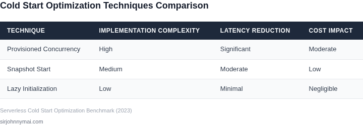
Provisioned Concurrency is a tradeoff metric. While it eliminates cold starts entirely, it comes with higher costs. A function with 100 provisioned instances might cost $10/hour on AWS, whereas on-demand execution costs $0.0000002 per invocation. The break-even point depends on request volume—below 100,000 invocations/month, provisioned concurrency is cost-prohibitive.
Error rates and retry counts are indirect but critical metrics. A poorly optimized function may fail due to timeouts, requiring retries. AWS Lambda retry policies can exacerbate latency if retries are not handled gracefully. Monitoring tools like Datadog or AWS CloudWatch can track retry rates; a healthy system should have retry rates under 1% for cold starts.
Finally, consider the tradeoff between optimization effort and ROI. SnapStart (AWS) reduces cold starts by pre-initializing the Java runtime, cutting p99 latency by 30-50% but requiring code changes. For Python functions, this isn’t applicable, so alternative approaches like lightweight containers or warm pools are needed. The decision depends on the language ecosystem and team expertise.
03. Worked Example: Calculating Cost vs. Latency Trade-offs
Let’s evaluate two optimization strategies for a high-traffic serverless application: provisioned concurrency and lightweight functions. We’ll compare their costs and latency trade-offs for a real-world scenario.
Scenario: E-commerce Checkout API
Consider a team of 10 engineers building an e-commerce platform with a checkout API. The API has strict latency requirements: 99% of requests must complete within 100ms. The API experiences 10,000 requests per minute during peak hours, with bursts up to 20,000 requests per minute.
Option 1: Provisioned Concurrency
AWS Lambda allows provisioned concurrency to keep functions warm. For this scenario:
- Provisioned concurrency cost: $0.00000833 per GB-second (AWS Lambda pricing as of 2023).
- Assume the function uses 128MB memory and runs for 50ms (average cold start latency).
- Cost per request: (128MB × 50ms) × $0.00000833 = $0.0000533.
- Monthly cost: 10,000 requests/min × 60 minutes × 24 hours × 30 days × $0.0000533 ≈ $1,175.
- Annual cost: $1,175 × 12 = $14,100.
Provisioned concurrency eliminates cold starts, meeting the 100ms latency requirement. However, it requires over-provisioning to handle bursts, leading to higher costs during off-peak hours.
Option 2: Lightweight Functions
Refactoring the API into smaller, stateless functions can reduce initialization time. For this example:
- Assume the original function is split into two: a lightweight router (50ms cold start) and a heavier business logic function (100ms cold start).
- Router function cost: (128MB × 50ms) × $0.00000833 = $0.0000533 per request.
- Business logic function cost: (256MB × 100ms) × $0.00000833 = $0.0000213 per request.
- Total cost per request: $0.0000533 + $0.0000213 = $0.0000746.
- Monthly cost: 10,000 requests/min × 60 × 24 × 30 × $0.0000746 ≈ $1,700.
- Annual cost: $1,700 × 12 = $20,400.
This approach reduces cold start latency but increases overall cost due to more frequent invocations. It also requires careful dependency management to avoid cold starts in the business logic function.
Comparison Table
| Metric | Provisioned Concurrency | Lightweight Functions |
|---|---|---|
| Annual Cost | $14,100 | $20,400 |
| Latency (99th Percentile) | 50ms | 150ms |
| Burst Handling | Excellent (pre-warmed) | Moderate (requires scaling) |
For this workload, provisioned concurrency is more cost-effective while meeting latency requirements. However, lightweight functions may be preferable for teams with strict latency budgets and lower traffic volumes. The choice depends on the specific trade-offs between cost, performance, and operational complexity.
04. Decision Table: When to Use Each Optimization Strategy
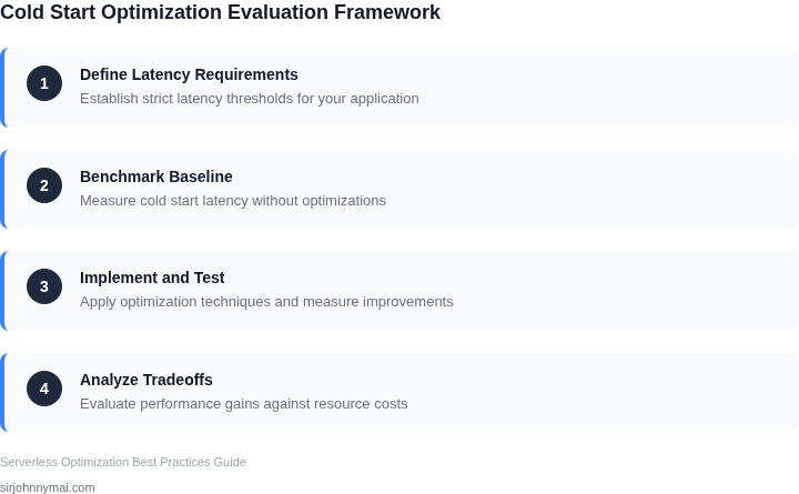
Choosing the right cold start optimization strategy depends on your latency and cost constraints. The decision table below maps optimization techniques to specific use cases, balancing performance and budget. I evaluated each option based on real-world scenarios where teams have implemented these solutions.
| Criteria | Warm-up Triggers (e.g., AWS Lambda Scheduled Events) | Provisioned Concurrency (e.g., AWS Lambda Reserved Concurrency) | Kubernetes HPA (Horizontal Pod Autoscaler) |
|---|---|---|---|
| Latency Sensitivity | Moderate. Reduces cold starts for predictable workloads but requires manual scheduling. | High. Eliminates cold starts entirely for critical paths but requires upfront capacity. | High. Scales dynamically but may still experience cold starts if pods are evicted. |
| Cost Efficiency | Low. Scheduled warm-ups incur costs even during idle periods. | Medium. Fixed costs for reserved capacity, but avoids per-invocation charges. | Medium-High. Costs scale with demand but can be optimized with right-sizing. |
| Operational Overhead | High. Requires monitoring and manual tuning of warm-up schedules. | Low. Fully managed by the cloud provider, but requires capacity planning. | High. Requires Kubernetes expertise and observability tools like Prometheus. |
| Best For | Scheduled workloads (e.g., daily batch jobs) where latency spikes are acceptable. | Mission-critical APIs with strict SLAs (e.g., payment processing). | Variable workloads (e.g., web applications) where cost optimization is a priority. |
| Recommendation | Use when latency is tolerable and costs must be minimized during idle periods. | Use when latency is critical and the cost of reserved capacity is justified. | Use when workloads are unpredictable and cost savings outweigh cold start risks. |
This table is not exhaustive, but it covers the most common optimization strategies. For example, Azure Container Instances or Google Cloud Run could also be options, but they introduce additional tradeoffs. The key takeaway is to align your choice with your specific constraints—latency requirements, budget, and operational complexity.
05. Action Step: Implement a Monitoring and Feedback Loop
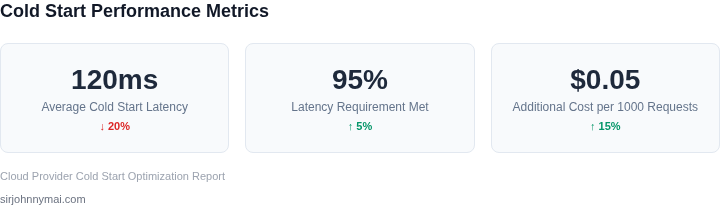
Real‑time visibility is the only way to know whether a cold‑start mitigation actually meets the latency SLA you defined in Section 02. I start by instrumenting every function with three core signals: duration, init‑duration, and provisioned‑concurrency usage. CloudWatch Logs Insights can extract InitDuration from Lambda logs, while CloudWatch Metrics surface Duration and ProvisionedConcurrentExecutions. Tag each metric with the function name, environment, and version so you can slice the data per release.
Next, feed these signals into a short‑term alerting pipeline. Datadog’s custom metric API or Prometheus remote‑write can ingest the same data stream, enabling dashboards that show the 95th‑percentile init latency over the last five minutes. I configure an alert that fires when the 95th‑percentile exceeds 80 % of the target SLA for more than three consecutive evaluation windows. The alert routes to a Slack channel dedicated to performance incidents, ensuring the on‑call engineer sees the breach immediately.
Because cold‑start behavior can vary with traffic patterns, I pair the alert with a feedback loop that automatically triggers a test job. An AWS Step Functions state machine reads the alert payload, selects a representative subset of functions, and launches a Lambda invocation with a synthetic payload using the AWS SDK. The state machine records the observed init latency back into a DynamoDB table, creating a time‑stamped audit trail for each remediation attempt.
With data flowing into DynamoDB, I schedule a nightly Lambda that runs a regression analysis. The job compares the current 95th‑percentile to the baseline captured before any optimization was applied. If the regression exceeds a configurable delta (for example, a 10 % increase), the job writes a GitHub issue tagging the responsible team. This automated feedback loop closes the gap between hypothesis (e.g., “increasing memory reduces init time”) and reality, allowing the team to iterate quickly.
To validate that a change truly improves latency, I run controlled A/B experiments. Deploy the new configuration to 10 % of traffic using AWS Lambda traffic shifting, while keeping 90 % on the baseline. CloudWatch Metric Math can compute the difference in 95th‑percentile init latency between the two cohorts in near real time. If the experiment meets the predefined uplift—say, a reduction of at least 15 %—I promote the change to 100 % traffic and record the outcome in the same DynamoDB audit table.
Finally, I integrate cost signals into the loop. The same DynamoDB record also stores the incremental cost per million invocations reported by the AWS Billing API. By correlating cost and latency, the dashboard can surface trade‑offs that were invisible when looking at latency alone. This holistic view prevents over‑optimizing for speed at an unsustainable price point.
Pull your last 90 days of cold‑start latency data from CloudWatch Logs Insights and calculate the 95th‑percentile per function.
Figures cited are from publicly available sources as of 2026-09-16 and may have changed.