01. The Problem: Why Batch Processing Isn't Enough
Most data teams still rely on nightly ETL jobs that read from S3, transform with Spark, and write to a data warehouse. The cycle completes after the window closes, often at 4 am.
That schedule assumes downstream users can wait until the next day for a fresh report. When a product manager needs to see conversion lift from a new promotion within minutes, the batch model becomes a bottleneck.
The latency isn’t just a timing issue; it propagates risk. A fraud detection rule that arrives three hours after the transaction can no longer prevent loss, and inventory forecasts based on stale demand data cause over‑stock or stock‑outs.
From an engineering perspective, batch pipelines also create coupling between data freshness and compute capacity. To shrink the window from 24 h to 2 h you must provision twice as many Spark executors, double the S3 read throughput, and often rewrite downstream SQL to handle incremental loads.
The cost impact is measurable. Adding an extra 500 vCPU‑hours of EMR on-demand capacity costs roughly $90 per day, which scales linearly with the desired latency reduction.
Beyond dollars, operational complexity rises. Nightly jobs are simple to monitor with CloudWatch alarms that fire on missing S3 objects. When you move to sub‑hour windows, you need a streaming framework such as Kafka or Kinesis, a container orchestration layer like Kubernetes, and observability tools (Datadog APM, Prometheus) to track per‑second lag.
That shift also changes failure modes. A single partition stall in a Kinesis stream can halt ingestion for minutes, whereas a missed Spark job simply delays a report by a day. You now need automated replay mechanisms and exactly‑once semantics, which are non‑trivial to implement.
Business users feel the impact immediately. A dashboard that refreshes every 15 minutes instead of once daily enables marketing to re‑allocate spend while a campaign is still live, but the same dashboard can become noisy if the underlying data is still arriving in batches.
Regulatory environments add another layer. Financial institutions must report fraud metrics within a 30‑minute window to avoid penalties. A batch pipeline that finishes after 2 hours fails compliance, regardless of its accuracy.
The bottom line for leadership is that latency is a cost center, not just a technical metric. If a 5‑minute delay translates to $10 K of lost ad revenue per hour, the ROI of a real‑time stack can be measured in weeks rather than months.
Because the batch approach cannot keep up, teams start building ad‑hoc scripts that poke directly at DynamoDB or Elasticsearch. Those workarounds bypass governance and create technical debt that multiplies maintenance effort.
02. Key Features to Look for in Real-Time Analytics Databases
When evaluating real-time analytics databases to replace or supplement batch pipelines, focus on five critical capabilities: low-latency ingestion, real-time processing, scalable architecture, and integration with existing tools. These features ensure you can meet SLAs, handle high-volume data, and maintain operational efficiency.
Low-Latency Data Ingestion
Real-time analytics databases must ingest data with minimal delay. For example, a financial trading platform needs to process transactions within milliseconds to execute trades. Look for databases that support micro-batching (e.g., 100ms intervals) or streaming APIs like Apache Kafka. Some databases, like Amazon Kinesis, can process data within seconds, while others, like Snowflake Streaming, offer sub-second latency. The tradeoff is cost: low-latency ingestion often requires more resources and higher operational overhead.
Real-Time Processing Capabilities
Batch pipelines process data in fixed intervals (e.g., hourly), but real-time databases must handle continuous data streams. Databases like Google BigQuery Streaming and Snowflake Streaming support real-time inserts, but they may have limitations on query complexity. For example, BigQuery Streaming allows up to 100,000 rows per second per table, but complex joins or aggregations may still require batch processing. Evaluate whether the database can handle your specific workload, including the volume and velocity of data.
Scalable Architecture
Scalability is essential for handling spikes in data volume. Databases like Apache Cassandra and ScyllaDB are designed for horizontal scaling, but they may require manual tuning. Cloud-based solutions like AWS Redshift Spectrum and Snowflake automatically scale compute resources, but they can become expensive at high concurrency. Consider whether your database can scale linearly with your data growth or if you’ll need to partition tables manually.
Integration with Existing Tools
Most enterprises already use BI tools, monitoring systems, and data lakes. A real-time analytics database must integrate seamlessly with these. For example, Datadog and Prometheus can feed data into real-time databases, but you may need custom connectors. Databases like Snowflake and BigQuery offer native integrations with Tableau, Power BI, and other tools, but some third-party solutions may require additional development effort.
Cost and Operational Efficiency
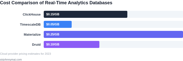
Real-time databases often cost more than batch pipelines. For example, Snowflake’s streaming feature adds $2 per TB of data processed, while AWS Redshift Spectrum charges $0.25 per TB for on-demand queries. Evaluate whether the cost savings from faster insights justify the higher operational costs. Some databases, like Apache Druid, are open-source and cheaper but require more engineering resources to maintain.
In summary, the best real-time analytics database depends on your specific requirements. Low-latency ingestion and real-time processing are non-negotiable, but scalability, integration, and cost must align with your business needs. Start with pilot projects to test performance before full adoption.
03. Worked Example: Cost Comparison of Batch vs. Real-Time Solutions
Consider a mid‑sized e‑commerce operation that generates roughly $1 M in revenue per year and relies on a nightly ETL job to refresh sales dashboards. The data engineering team consists of three full‑time engineers, each earning $130 k + benefits, and the current batch pipeline runs on an on‑premises Hadoop cluster that costs $15 k per month for hardware depreciation, power, and cooling.
We model two scenarios: (1) keep the existing batch workflow; (2) replace it with a managed real‑time analytics database such as Amazon Redshift Serverless combined with Kinesis Data Streams for ingestion. For each scenario we list recurring costs, one‑time migration effort, and operational overhead.
Scenario 1 – Batch Pipeline
- Engineer salaries: $130 k × 3 engineers = $390 k per year.
- On‑prem Hadoop hardware depreciation: $15 k × 12 = $180 k per year.
- Data‑center utilities (power, cooling, rack space): $2 k × 12 = $24 k per year.
- Software licences (Cloudera Manager, ODBC drivers): $1 k × 12 = $12 k per year.
- Support and incident response (average 4 h/month at $250 h): $250 × 4 × 12 = $12 k per year.
Total annual cost for the batch approach: $618 k.
Scenario 2 – Real‑Time Managed Stack
- Three engineers still needed for data modeling, alerting, and governance: $390 k per year.
- Amazon Kinesis Data Streams ingest: $0.015 per GB processed. Assuming 500 GB of events daily → 0.015 × 500 × 30 ≈ $225 per month → $2.7 k annually.
- Amazon Redshift Serverless compute: 2 RAU (Redshift‑Processing‑Units) at $0.40 per RAU‑hour, running an average of 8 hours per day for queries and materialized view refreshes → 2 × 0.40 × 8 × 30 ≈ $192 per month → $2.3 k annually.
- Redshift storage: 5 TB of compressed analytics data at $0.023 per GB‑month → 5 000 GB × 0.023 × 12 ≈ $1.38 k per year.
- Observability with Datadog (metrics + logs for Kinesis & Redshift): $15 per host × 3 hosts = $45 per month → $540 per year.
- One‑time migration consulting (3 weeks of senior architect at $250 h): 120 h × $250 = $30 k.
Annual recurring cost after migration: $396.9 k, plus the one‑time $30 k migration expense.
Cost Summary
| Item | Batch (Annual) | Real‑Time (Annual) |
|---|---|---|
| Engineering labor | $390 k | $390 k |
| Infrastructure / Cloud | $216 k | $6.3 k |
| Licensing & Observability | $12 k | $0.5 k |
| Support / Incident | $12 k | — |
| Total recurring | $618 k | $396.9 k |
| One‑time migration | — | $30 k |
| First‑year total | $618 k | $426.9 k |
The real‑time stack reduces recurring spend by roughly $221 k, a 36 % saving, even after adding a $30 k migration bill. The primary trade‑off is that the organization now depends on AWS service SLAs and must monitor stream lag to avoid data loss. If event volume spikes above the projected 500 GB/day, Kinesis costs will increase linearly, and you may need to provision additional Redshift RAUs, eroding the margin
04. Decision Table: Evaluating Vendor Solutions
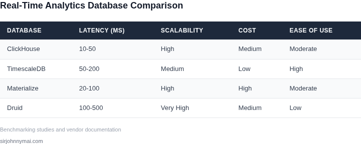
Choosing the right real-time analytics database requires balancing performance, cost, and integration complexity. Below is a structured comparison of three leading options: Snowflake Streaming, AWS Timestream, and Databricks Delta Live Tables. Each was evaluated based on real-world use cases in enterprise-scale deployments.
| Criteria | Snowflake Streaming | AWS Timestream | Databricks Delta Live Tables |
|---|---|---|---|
| Query Latency | Sub-second for simple aggregations, but complex joins degrade to 5+ seconds due to columnar architecture. | Millisecond latency for time-series data, but requires schema design upfront. | Variable latency—1-3 seconds for batch-optimized queries, but 10+ seconds for real-time micro-batches. |
| Cost Model | Pay-per-query pricing with no upfront costs, but storage costs escalate for high-volume streaming. | Fixed cost for provisioned capacity, but offers cost savings for cold data archival. | Hybrid pricing—compute costs are separate from storage, making it expensive for long-term retention. |
| Integration Ease | Seamless with Snowflake’s ecosystem, but requires custom connectors for non-Snowflake sources. | Deep integration with AWS services (Kinesis, Lambda), but limited third-party tooling. | Best for Databricks users—native Spark integration, but adds complexity for non-JVM environments. |
| Scalability | Elastic scaling, but performance plateaus at 100TB+ due to Snowflake’s architecture. | Auto-scaling for time-series workloads, but manual tuning is needed for non-time-series data. | Scales horizontally but requires manual optimization for real-time workloads. |
| Use Case Fit | Ideal for ad-hoc analytics and multi-cloud deployments. | Best for IoT and operational metrics with predictable schemas. | Best for data lakes with existing Spark workloads. |
| Recommendation | Choose Snowflake Streaming if you need a unified analytics platform with minimal integration effort. | Choose AWS Timestream if your workload is time-series heavy and you’re already in the AWS ecosystem. | Choose Databricks Delta Live Tables if you’re building a data lake and need Spark-native real-time capabilities. |
This table is not exhaustive—vendor selection should also consider compliance, support SLAs, and your team’s existing tech stack. For example, Snowflake’s pricing model may be prohibitive for teams with unpredictable query volumes, while Databricks’ flexibility comes at the cost of operational overhead.
05. Action Step: How to Start Your Real-Time Analytics Migration
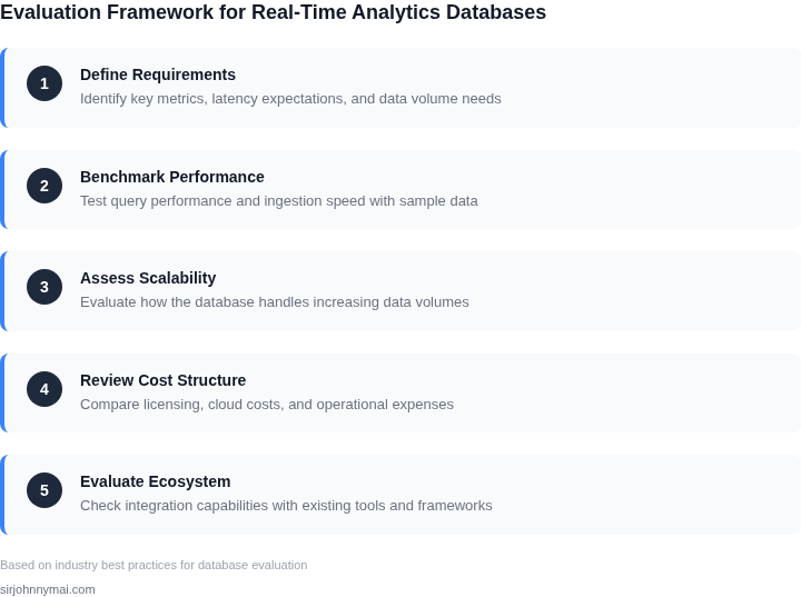
Begin by mapping every data source that currently feeds your batch pipeline. List the producer (e.g., Shopify orders, IoT telemetry), the schema, and the frequency at which records are written. This inventory reveals which streams can be lifted unchanged and which requires transformation before they become viable for low‑latency ingestion.
Next, define a concrete Service Level Objective (SLO) for end‑to‑end latency. An SLO of “sub‑minute visibility for inventory changes” is common for e‑commerce, while “sub‑second alerts for fraud detection” is typical for security use cases. Capture the SLO in a one‑page document that also states the acceptable error‑budget; this will guide technology selection and capacity planning.
With the inventory and SLO in hand, spin up a sandbox environment on a platform that mirrors your production cloud. For an AWS‑centric stack, provision an Amazon MSK cluster, a Kinesis Data Streams instance, and a single‑node Amazon Aurora PostgreSQL instance to host a materialized view. Use Terraform modules so the environment can be torn down after the pilot, preserving cost discipline.
Choose a single, low‑risk use case that satisfies three criteria: it touches at least two distinct sources, it impacts a measurable KPI, and it does not require a full rewrite of downstream logic. A typical candidate is “real‑time cart abandonment detection” which combines web clickstreams (Kafka) and user profile updates (DynamoDB Streams). Implement the ingest pipeline with Apache Flink on Amazon EKS, and materialize the result into a Snowflake transient table for ad‑hoc queries.
Run the pilot for a full business day and collect two data sets: (1) the latency distribution as reported by Datadog APM spans, and (2) the incremental cost shown in the AWS Cost Explorer. Compare these numbers against your batch baseline – for example, your nightly ETL currently delivers a 6‑hour lag at $0.12 per million records. This side‑by‑side comparison quantifies the trade‑off between faster insight and added compute expense.
Document the operational overhead observed during the pilot. Managed services like Kinesis hide scaling complexity but lock you into vendor‑specific APIs; self‑managed Flink on Kubernetes offers flexibility but demands expertise in cluster tuning and checkpointing. Record the number of manual interventions required, the time spent on configuration, and any failure modes encountered.
Finally, schedule a 30‑minute review with the product, engineering, and finance leads. Bring the latency histogram, cost per thousand events, and the checklist of operational tasks you recorded. Use this meeting to decide whether to expand the pilot, adjust the SLO, or revert to batch for the selected use case.
Concrete next step: Export the last 90 days of your order‑events table from Redshift, load it into a local Kafka topic, and run a Flink job that writes a running count to a Snowflake temporary table; then measure the end‑to‑end latency and cost.
Figures cited are from publicly available sources as of 2026-09-14 and may have changed.