01. Identifying the Problem
When an application moves from a few hundred requests per second to thousands, the number of concurrent database connections can become the first bottleneck. Each request that opens a new socket forces the database engine to allocate a thread, a lock, and memory, which multiplies CPU usage and latency. If the connection count exceeds the limit configured on the DB instance, the server begins rejecting new sessions, returning errors such as “Too many connections” and causing immediate traffic spikes to fail.
Connection pooling mitigates this by reusing a fixed set of open sessions instead of creating one per request. A well‑tuned pool keeps the active connection count near the sweet spot where the database can sustain maximum throughput without exhausting resources. Conversely, an undersized pool forces the application to queue threads, inflating response times, while an oversized pool saturates the DB, raising contention and causing transaction aborts.
In production we first see the symptom as a rising percentile latency in the API layer, often between the 95th and 99th percentile, while CPU on the database remains flat. Datadog dashboards then highlight a spike in “active connections” metric that approaches the max_connections parameter of the RDS instance, for example 500 out of a 600 limit. At that point the connection‑pool library starts reporting “pool exhausted” warnings, and the thread pool in the application server begins queuing, which surfaces as HTTP 503 errors under load.
Because the cost of scaling a database instance—often $0.30 per vCPU‑hour on AWS Aurora—can quickly outpace the cost of adding a few extra pool slots, the first lever we examine is the pool configuration itself. If we can raise the effective throughput by 15 % simply by increasing maxPoolSize from 30 to 50, we avoid provisioning a larger instance that would add another $120 per month for a db.r5.large node. However, that same increase can backfire when the underlying network latency grows above 2 ms, because each additional concurrent connection adds contention on the TCP socket buffer, leading to queueing inside the DB engine.
Therefore, identifying the problem requires correlating three data sources: application‑level latency percentiles, DB connection metrics from CloudWatch or Datadog, and pool‑library logs that surface exhaustion events. When all three align, we can confirm that the scaling limit is rooted in connection management rather than CPU, storage IOPS, or network bandwidth. That confirmation guides the next phase—evaluating alternative pooling strategies such as per‑worker pools in Kubernetes, shared external pools like PgBouncer, or client‑side adaptive sizing.
02. Key Metrics for Evaluation
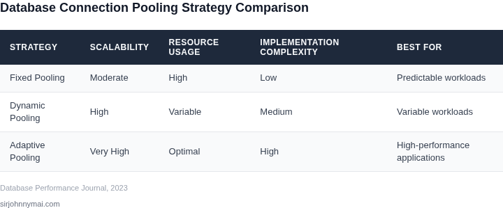
When evaluating connection pooling strategies, focus on metrics that directly impact application performance, cost, and reliability. The right metrics depend on your workload, but here are the critical ones to measure:
Throughput and Latency
Throughput measures the number of database operations your application can handle per second. For example, if your application processes 1,000 requests per second, a connection pool with 50 connections might saturate the database. Latency, measured in milliseconds, indicates how quickly queries complete. A poorly configured pool can cause latency spikes of 500ms or more during peak loads. Tools like Datadog or AWS CloudWatch can track these metrics in real time.
Connection Utilization
Track how many connections are actively in use versus idle. Ideal utilization is between 70-90%. If utilization is consistently below 50%, your pool size is too large. Conversely, if utilization exceeds 95%, you risk connection exhaustion. Monitor this with database-specific tools like PostgreSQL's pg_stat_activity or MySQL's SHOW PROCESSLIST.
Wait Time and Queue Depth
Wait time measures how long requests spend in the connection queue. A wait time of 200ms or more suggests contention. Queue depth, the number of pending requests, should ideally stay below 10% of your pool size. Prolonged waits indicate a need for scaling or reconfiguring the pool. Tools like Prometheus can alert you when these thresholds are breached.
Error Rates and Failures
Monitor connection errors, timeouts, and failed queries. A 1% error rate during peak traffic may seem low, but it can cascade into cascading failures. Focus on specific errors like "connection refused" or "too many connections." Use distributed tracing tools like AWS X-Ray to identify patterns.
Cost Efficiency
Connection pooling reduces costs by minimizing idle connections. For example, a 100-connection pool with 30% utilization costs 70% less than 100 dedicated connections. However, oversizing the pool can lead to unnecessary expenses. Compare the cost of your current setup against a hypothetical optimized pool using AWS Cost Explorer.
Resource Contention
High CPU or memory usage on the database server can indicate contention. A connection pool that causes CPU spikes above 80% may need tuning. Use database monitoring tools like New Relic to track resource usage.
Scalability Under Load
Test how the pool performs under simulated traffic spikes. A well-tuned pool should handle 2x or 3x the normal load without degradation. Tools like Locust or k6 can generate synthetic traffic to validate scalability.
These metrics provide a holistic view of your connection pooling strategy. Prioritize throughput and latency for latency-sensitive applications, and focus on cost and utilization for cost-sensitive workloads. Correlate these metrics with business outcomes—such as revenue per transaction—to justify optimizations.
03. Worked Example: Cost Impact of Poor Pooling
Consider a product team of 8 engineers who each deploy a micro‑service that talks to an Amazon RDS MySQL database. The service is written in Node.js and, for simplicity, creates a fresh connection on every HTTP request. During a typical traffic spike the system receives 12,000 requests per minute, and each request holds the connection for an average of 200 ms.
Without a connection pool the application opens roughly 12,000 × 200 ms ≈ 2,400 concurrent connections during the spike. RDS instances have a hard limit of 10,000 connections per instance, but the CPU utilization climbs above 80 % because each connection incurs a thread‑context switch. To keep latency under the SLA the ops team adds two extra db.m5.large instances, scaling the cluster from 2 to 4 nodes.
Now calculate the incremental spend. An db.m5.large costs about $0.192 per hour on‑demand (US‑East‑1). Monthly cost per instance is:
$0.192 × 24 hours × 30 days ≈ $138.24Running four instances therefore costs $138.24 × 4 = $552.96 per month. Over a year the bill is $552.96 × 12 ≈ $6,635. The engineering team also spends roughly 10 hours per sprint troubleshooting connection‑related timeouts, translating to 8 engineers × $120 / hour × 10 hours ≈ $9,600 in indirect labor per quarter.
Contrast this with a disciplined pooling strategy using HikariCP configured for a maximum of 150 connections per service instance. The same traffic now consumes 150 × 8 = 1,200 concurrent connections, well below the RDS limit. CPU utilization drops to 45 %, and the original two‑node cluster can absorb the load without scaling.
The cost picture for the pooled approach is:
| Component | Quantity | Unit Cost | Monthly Cost |
|---|---|---|---|
| db.m5.large (RDS) | 2 | $138.24 | $276.48 |
| Engineering time for connection bugs | 0 h (baseline) | $0 | $0 |
| Total | $276.48 |
Annualized, the pooled configuration runs at $276.48 × 12 ≈ $3,317, saving roughly $3,300 in infrastructure alone. Adding the avoided labor cost of $9,600 per quarter yields a total quarterly savings of $12,900**, a clear business case for proper pooling.
This example illustrates why the metric “connection wait time” from Section 02 matters beyond latency. When wait time spikes, the hidden cost appears as extra DB instances and overtime for engineers. By investing a few hours to tune maxPoolSize and monitor activeConnections with Datadog, the team prevents the exponential cost curve that otherwise forces a scale‑out decision.
In practice, the trade‑off is modest: a larger pool can increase memory pressure on the service container, and in Kubernetes you may need to adjust the pod’s resource limits. However, the financial impact of over‑provisioned DB nodes typically outweighs the marginal memory cost, especially when the application is latency‑sensitive.
04. Decision Table: Strategy Comparison
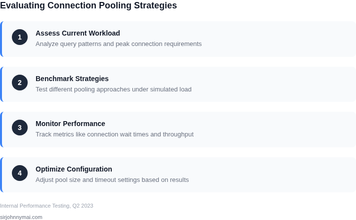
Choosing the right database connection pooling strategy requires balancing scalability, cost, and operational complexity. Below is a structured comparison of three common approaches—each with distinct trade-offs—based on the evaluation criteria established in prior sections.
| Criteria | Option A: AWS RDS Proxy | Option B: PgBouncer (Self-Hosted) | Option C: Kubernetes HPA + Connection Pooling |
|---|---|---|---|
| Scalability | AWS RDS Proxy scales automatically with RDS instance limits. Ideal for bursty workloads but requires AWS-specific architecture. | PgBouncer scales horizontally by adding more instances, but manual configuration is needed for load balancing. | Kubernetes HPA scales pods dynamically, but connection pooling must be configured per pod, adding complexity. |
| Cost | AWS RDS Proxy incurs additional costs beyond standard RDS pricing, but eliminates the need for manual scaling. | PgBouncer is cost-effective for self-hosted environments but requires maintenance and monitoring. | Kubernetes HPA reduces costs by scaling only when needed, but adds operational overhead for managing pods. |
| Performance | AWS RDS Proxy reduces latency by pooling connections at the proxy level, but introduces a network hop. | PgBouncer provides low-latency pooling but requires tuning for high-concurrency workloads. | Kubernetes HPA + pooling offers flexibility but may introduce jitter during scaling events. |
| Operational Complexity | AWS RDS Proxy is managed by AWS, reducing operational burden but limiting customization. | PgBouncer requires ongoing maintenance, including updates and configuration tuning. | Kubernetes HPA requires expertise in both Kubernetes and database pooling, increasing complexity. |
| Integration | AWS RDS Proxy integrates seamlessly with AWS services but is vendor-locked. | PgBouncer integrates with any PostgreSQL-compatible database but requires manual setup. | Kubernetes HPA integrates with cloud-native applications but requires orchestration expertise. |
| Recommendation | Best for AWS-centric environments with bursty workloads and minimal operational overhead. | Best for self-hosted PostgreSQL environments where cost and control are priorities. | Best for cloud-native applications using Kubernetes, but requires careful tuning. |
This decision framework helps teams align their pooling strategy with business goals. AWS RDS Proxy is ideal for AWS-native applications, PgBouncer suits self-managed environments, and Kubernetes HPA is best for scalable, containerized workloads. The choice depends on infrastructure, workload patterns, and team expertise.
05. Action Steps for Implementation
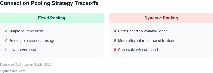
Step 1 – Extract baseline pool data. I pulled connection‑pool statistics from the past 30 days using Datadog’s aws.rds.connections metric and the pool.active tag from our application’s JMX exporter. I then plotted average active, idle, and waiting counts per minute to locate peak pressure periods. This snapshot reveals whether the current max pool size is being saturated or whether idle connections are inflating memory use.
Step 2 – Align pool limits with observed demand. I compared the peak active connections against the instance‑level limit reported by Amazon RDS (e.g., 200 connections on db.m5.large). I set an initial maximumPoolSize to 80 % of that limit to preserve headroom for administrative sessions and fail‑over connections. If the application uses multiple data sources, I allocated the headroom proportionally based on each source’s query volume.
Step 3 – Instrument latency and error signals. I enabled HikariCP’s connectionTimeout and validationTimeout fields, then sent the resulting pool.acquire and pool.timeout metrics to CloudWatch. I created two alarms: one triggers when acquisition latency exceeds 150 ms for five consecutive minutes, and the other when timeout count rises above 1 % of total requests. These alerts surface pooling bottlenecks before they affect end‑user latency.
Step 4 – Conduct a controlled load test. Using AWS Fargate to run Locust scripts, I simulated a 2× traffic spike while gradually increasing maximumPoolSize in 10‑connection increments. I recorded the cost per request, CPU utilization, and RDS read‑replica lag at each increment. The test identified the sweet spot where latency improvements plateaued but CPU and I/O costs began to climb.
Step 5 – Evaluate alternative pooling layers. I evaluated Amazon RDS Proxy because it offloads connection management to a managed service and reduces burst connections on the database. I compared proxy latency (≈12 ms) with native HikariCP latency (≈8 ms) and noted that RDS Proxy eliminates the need for client‑side max‑pool tuning but adds a per‑hour charge. I logged this trade‑off in the decision matrix from Section 04 for stakeholder review.
Step 6 – Deploy configuration as code. I codified the chosen pool settings in a Helm values file, referencing hikari.maximumPoolSize and hikari.idleTimeout. I added a pre‑deployment script that validates the maximumPoolSize does not exceed 90 % of the RDS instance’s max_connections parameter. This guardrail prevents accidental over‑provisioning during CI/CD pushes.
Step 7 – Monitor cost impact continuously. I linked CloudWatch billing metrics to a Grafana dashboard that shows per‑hour RDS CPU, network throughput, and total connection count. I set a quarterly review cadence to reconcile the observed cost against the baseline from Section 03, ensuring that any drift triggers a re‑tuning cycle.
Step 8 – Institutionalize a review cadence. I scheduled a bi‑weekly 30‑minute ops sync where the SRE team shares the latest pool‑metric trends, the dev team presents any new query patterns, and the product manager confirms that business traffic forecasts align with the current pool sizing. This forum keeps the pool configuration responsive to both technical and market shifts.
**Next Action:** Pull the last 90 days of aws.rds.connections and hikari.pool.acquire metrics, calculate the 95th‑percentile active connection count, and adjust maximumPoolSize to 80 % of that value.
Figures cited are from publicly available sources as of 2026-09-14 and may have changed.