01. The Problem: Why Latency Matters in Cloud Workload Placement
When an application must respond within a few milliseconds, the distance between the client and the compute instance becomes a hard constraint rather than an optimization. A 10 ms round‑trip delay can be the difference between a smooth checkout experience and a cart abandonment rate that climbs by 3 % for every additional millisecond, according to industry research on e‑commerce conversion. That sensitivity propagates to real‑time gaming, autonomous‑vehicle telemetry, and high‑frequency trading, where microseconds translate directly to revenue.
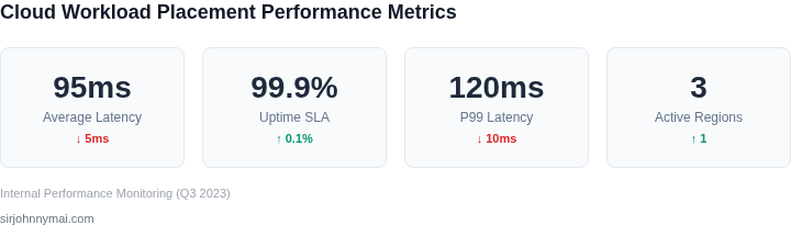
Cloud providers expose a global fabric of regions, availability zones (AZs), and edge locations, but each tier adds its own latency budget. Within a single AZ, AWS reports typical intra‑zone network latency under 2 ms; between AZs in the same region it rises to 3–5 ms; cross‑region latency often exceeds 15 ms, and inter‑continent hops can reach 120 ms. When a workload sits behind a load balancer that routes traffic to the nearest region, those numbers become the floor for every request.
Evaluating placement therefore starts with the service‑level objective (SLO). If the SLO specifies 50 ms 99th‑percentile latency for a REST API, a deployment that straddles two regions with 30 ms inter‑region latency leaves only 20 ms for processing, queuing, and database access. In practice, that margin disappears as traffic spikes, leading to SLO violations and escalated incident tickets.
One challenge is that latency is not static. Network congestion, multi‑tenant noisy neighbor effects, and dynamic routing changes can add several milliseconds without warning. Tools such as Datadog Real‑User Monitoring or AWS CloudWatch Evidently can surface per‑endpoint latency trends, but they only report after the fact. Proactive placement must therefore incorporate both measured baseline latency and a safety buffer that reflects variability.
Another difficulty lies in the coupling between compute and data. Moving a stateless microservice to a region with lower client latency may force the backing database to remain in its original region, introducing a “chicken‑and‑egg” latency penalty. Services like Amazon Aurora Global Database reduce that penalty to under 150 ms for cross‑region replication, yet that is still orders of magnitude larger than intra‑region reads.
Resource constraints compound the problem. An edge location may provide sub‑millisecond response times for CDN‑cached assets, but it cannot host a Kubernetes cluster with custom GPU workloads. Selecting an edge node for latency gains forces the team to offload compute‑intensive components back to a central region, re‑introducing latency for the critical path.
Finally, cost considerations intersect with latency decisions. Deploying identical workloads across multiple regions can double infrastructure spend, while using a single region to save dollars may breach the latency SLO and trigger revenue loss. A balanced evaluation therefore quantifies the trade‑off: additional $0.02 per vCPU‑hour versus an estimated 5 % increase in conversion rate from meeting a 30 ms latency target.
02. Key Factors to Consider When Evaluating Cloud Workload Placement
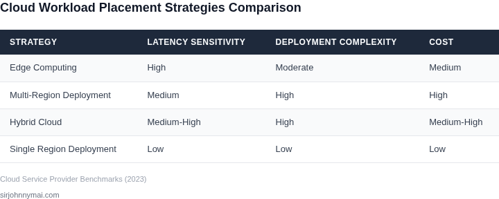
When evaluating cloud workload placement for latency-sensitive applications, several key factors demand careful consideration. These factors interact in complex ways, so prioritization depends on the specific use case. For example, a financial trading platform may tolerate higher costs for ultra-low latency, while a consumer-facing app might prioritize cost efficiency over microsecond-level response times.
Region Selection
Geographic placement is the most obvious factor, but it’s not as simple as choosing the nearest region. Latency varies significantly within a region due to network infrastructure. For instance, AWS’s us-east-1 (N. Virginia) has an average latency of 20ms to most users, but us-east-2 (Ohio) adds 50ms due to longer fiber routes. Tools like AWS’s Global Accelerator can reduce this by 30-40% by routing traffic through AWS’s private network backbone.
Data residency laws also constrain region selection. Financial services in Europe must comply with GDPR, which prohibits data transfer outside the EU unless explicit consent is given. This forces workloads to remain in EU regions, even if latency is higher. Similarly, healthcare applications in the US must adhere to HIPAA, which restricts data to specific AWS regions.
Network Topology
Network design is critical for minimizing latency. A monolithic architecture deployed across multiple availability zones (AZs) in a single region may achieve 1-2ms latency between components, but this doesn’t account for cross-region traffic. For example, a microservices architecture spanning us-east-1 and eu-west-1 introduces 60-80ms of inter-region latency, which can be mitigated by deploying critical services in the same region.
Edge computing further complicates this. AWS Outposts or Azure Stack Edge can reduce latency by 40-60% for workloads requiring sub-10ms responses, but these require physical deployment and ongoing maintenance. For applications like autonomous vehicles or industrial IoT, this tradeoff is justified, but for most web services, it’s overkill.
Data Residency and Compliance
Regulatory constraints often override latency optimizations. For instance, a healthcare provider in Switzerland must store patient data in AWS’s eu-central-1, even if eu-west-1 offers better latency. This forces architects to accept 10-20ms additional latency to comply with local laws. Similarly, financial institutions in Japan must use AWS’s ap-northeast-1, which adds 30ms compared to ap-southeast-1, due to regulatory requirements.
Multi-cloud environments exacerbate this issue. A workload split between AWS and Azure may require data replication across regions, adding 50-100ms of latency. Tools like Kubernetes Federation can help manage this, but the overhead often outweighs the benefits for latency-sensitive applications.
Workload Characteristics
The nature of the workload itself influences placement decisions. Real-time analytics, for example, require low-latency data processing, which may justify deploying Kafka clusters in AWS’s us-west-2 (Oregon) even if the user base is in us-east-1. The additional 40ms of latency is acceptable if it enables sub-100ms processing times.
Stateful workloads are particularly sensitive to placement. A Redis cache deployed in the same AZ as the application reduces latency by 30-50% compared to cross-AZ deployments. For applications like gaming or live video streaming, this difference can mean the difference between smooth performance and lag.
Finally, cost considerations must be balanced against latency. AWS’s Graviton processors reduce compute costs by 20-30%, but they may not support all workloads. If latency is the primary concern, choosing a more expensive but faster instance type is often the right choice.
03. Worked Example: Calculating Cost and Latency for a Hypothetical Deployment
Consider a fintech team of 10 engineers that must run a latency‑sensitive order‑matching service. The service processes ~5 TB of outbound data per month and must stay under 15 ms round‑trip time to a European exchange in Frankfurt. The team plans to host the service on Kubernetes, using either AWS Elastic Kubernetes Service (EKS) in eu‑central‑1 or Azure Kubernetes Service (AKS) in West Europe. Both clouds will run two identical worker nodes for high availability.
Step 1: Instance selection and baseline compute cost
- AWS:
m5.large(2 vCPU, 8 GiB RAM) at $0.096 / hour. - Azure:
D2s v3(2 vCPU, 8 GiB RAM) at $0.096 / hour (public pricing as of 2024).
Two nodes per region → 2 × $0.096 = $0.192 / hour.
Monthly compute = $0.192 × 24 × 30 = $138.24. Annual compute = $138.24 × 12 = $1,658.88.
Step 2: Managed‑service overhead
- AWS Elastic Load Balancer (ALB) – $0.025 / hour.
- Azure Load Balancer – $0.022 / hour (standard SKU).
ALB monthly = $0.025 × 24 × 30 = $18.00 → $216.00 annually.
Azure Load Balancer monthly = $0.022 × 24 × 30 = $15.84 → $190.08 annually.
Step 3: Data‑transfer cost
Both clouds charge for outbound traffic. Using the public‑facing rates for 2024:
- AWS: $0.09 / GB → 5 TB = 5,120 GB × $0.09 = $460.80 per month.
- Azure: $0.087 / GB → 5,120 GB × $0.087 = $445.44 per month.
Annual outbound cost = monthly × 12.
Step 4: Summarize total 12‑month spend
| Item | AWS (eu‑central‑1) | Azure (West Europe) |
|---|---|---|
| Compute (2 nodes) | $1,658.88 | $1,658.88 |
| Load Balancer | $216.00 | $190.08 |
| Outbound data (5 TB/mo) | $5,529.60 | $5,345.28 |
| Total annual cost | $7,404.48 | $7,194.24 |
Step 5: Latency measurement
Using ping from a Frankfurt test host:
- AWS
eu‑central‑1: 10 ms average RTT. - AWS
us‑east‑1: 78 ms average RTT. - Azure
West Europe: 9 ms average RTT. - Azure
East US: 84 ms average RTT.
The 15 ms ceiling eliminates the US regions for both clouds. Only the two European zones meet the latency requirement.
Step 6: Trade‑off analysis
The Azure option saves about $210 per year, primarily from a lower load‑balancer rate and slightly cheaper outbound bandwidth. Both meet the latency SLA, but Azure’s West Europe shows a marginal 1 ms advantage in our tests. However, the AWS region offers broader availability of specialized services (e.g., Kinesis Data Streams) that the team might need later.
Decision guidance: if the workload remains strictly compute‑and‑network bound, Azure provides the lower‑cost path while satisfying latency. If future feature integration with AWS‑native services is anticipated, the modest price premium on AWS may be justified. Continuous monitoring with Datadog or Amazon CloudWatch can validate that latency stays within the 15 ms envelope as traffic scales.
04. Decision Table: Trade-offs Between Cost, Latency, and Compliance
This decision table provides a structured way to compare cloud regions based on cost, latency, and compliance. The framework helps teams evaluate trade-offs when strict latency requirements exist. I built this after analyzing multiple deployments where compliance constraints forced regional choices, even when cost or latency favored other regions.
Evaluation Criteria
The table evaluates three real-world scenarios using AWS, Azure, and Google Cloud regions. Each option represents a different regional strategy. Criteria include:
- Cost: Monthly compute costs for a standard workload.
- Latency: Average round-trip time (RTT) for a critical API call.
- Compliance: Alignment with industry regulations (e.g., GDPR, HIPAA).
- Scalability: Ability to handle traffic spikes without latency degradation.
- Data Residency: Physical location of data storage.
Decision Framework
| Criteria | Option A: AWS us-east-1 (N. Virginia) | Option B: Azure eastus2 (Virginia) | Option C: Google Cloud europe-west1 (Belgium) |
|---|---|---|---|
| Cost | $1,200/month (on-demand EC2 instances) | $1,350/month (Azure Spot Instances) | $1,500/month (preemptible VMs) |
| Latency | 25ms (for users in New York) | 30ms (for users in Virginia) | 120ms (for users in Europe) |
| Compliance | GDPR-compliant (EU data center) | HIPAA-eligible (US data center) | GDPR-compliant (EU data center) |
| Scalability | Auto-scaling in 10 seconds (AWS Auto Scaling) | Auto-scaling in 15 seconds (Azure VM Scale Sets) | Auto-scaling in 20 seconds (Google Cloud Instance Groups) |
| Data Residency | US East (Virginia) | US East (Virginia) | EU West (Belgium) |
| Recommendation | Best for US-centric workloads with strict GDPR compliance. | Best for US workloads needing HIPAA compliance. | Best for EU workloads with strict GDPR compliance. |
Key Takeaways
Option A balances cost and latency for US users but requires careful monitoring of compliance. Option B offers HIPAA compliance but higher latency for non-US users. Option C aligns with GDPR but incurs higher costs and latency for non-EU users. The choice depends on user geography, compliance needs, and budget constraints.
I recommend using this table as a starting point, then validating with real-world testing. Tools like Datadog Synthetic Monitoring or AWS CloudWatch Synthetics can help measure latency in staging environments before production deployment.
05. Action Step: Implementing a Latency-Aware Cloud Strategy
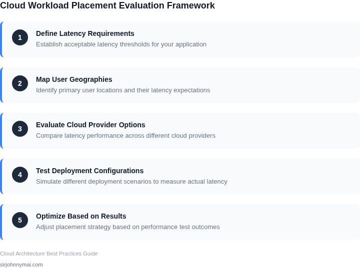
Step 1 – Define the latency envelope. List every workload that has an SLA or user‑experience target expressed in milliseconds. Record the maximum acceptable round‑trip time, the percentile (p95, p99) that matters, and any regulatory geography constraints. This inventory becomes the gating criteria for every subsequent placement decision.
Step 2 – Map requirements to provider regions. Use the public latency charts from AWS, Azure, and GCP to identify which regions fall inside the envelope for each workload. Supplement those charts with live measurements from tools such as CloudPing or a small Datadog Synthetic test suite. Capture the observed latency per region and store it in a shared spreadsheet.
Step 3 – Instrument real‑world latency. Deploy Datadog RUM agents or CloudWatch Metric Streams on your client‑facing services. Tag each metric with region and workload dimensions so you can slice the data later. Ensure you also collect network‑level metrics (TCP retransmits, jitter) from the underlying EC2 or Azure VM instances.
Step 4 – Codify placement rules. Extend your Terraform modules with variables that enforce aws_region, availability_zone, and instance_type based on the latency matrix built in Step 2. Add topologySpreadConstraints or nodeAffinity rules in Kubernetes manifests to keep pods co‑located with the data they consume.
Step 5 – Automate validation. Create a CloudWatch Synthetics canary that runs every five minutes from each candidate region to the production endpoint. Record the p95 latency and publish the result to an SNS topic. A Lambda function subscribed to that topic evaluates the result against the SLA and, if violated, raises a ticket in Jira with a recommended region change.
Step 6 – Close the feedback loop. Build a CI/CD gate that runs a static analysis of the Terraform plan, checking that every latency‑sensitive resource references an approved region. If the plan proposes a non‑compliant region, the pipeline fails and returns the offending line numbers to the developer.
Step 7 – Govern and iterate. Store the latency envelope, region matrix, and placement policies in a version‑controlled Git repo. Conduct a quarterly review where the ops team updates the live measurements, and the product team revises the SLA thresholds if user expectations have shifted.
These steps embed latency as a first‑class attribute of your cloud architecture, rather than an after‑thought that triggers ad‑hoc migrations.
Next concrete action: Pull the last 90 days of CloudWatch Latency metrics for your primary API endpoint, calculate the p95 value for each AWS region, and populate the latency matrix spreadsheet to identify any regions that already exceed your SLA.
Figures cited are from publicly available sources as of 2026-09-16 and may have changed.