01. The Problem: Bursty Traffic and Over-Provisioning
Bursty traffic patterns expose a fundamental tension between performance and cost. A single sudden surge can demand tenfold more compute than the baseline, yet that extra capacity sits idle for most of the day. The result is a “pay‑for‑nothing” scenario that erodes profitability.
Traditional capacity planning relies on historical averages, but bursty workloads—such as flash sales, news breaking, or gaming events—are rarely captured by a simple mean. Even sophisticated time‑series models can miss outliers that represent less than 1 % of total requests yet generate 30 % of peak load. Consequently, teams either under‑scale and suffer latency spikes, or they over‑scale to guarantee headroom.
Cloud providers charge per‑second for compute, so a 50 % over‑provisioned fleet can add up to $12,000 per month for a modest micro‑service running on 10 m5.large instances. That expense is invisible to developers until a quarterly budget review surfaces a variance of +27 % versus forecast. At the same time, over‑provisioned resources consume power and increase the organization’s carbon footprint, a metric increasingly scrutinized by investors.
Reactive autoscaling mechanisms, such as AWS Auto Scaling groups or Kubernetes Horizontal Pod Autoscaler, react after metrics cross a threshold, typically adding a new instance in 2–3 minutes. For latency‑sensitive APIs, a 150 ms cold‑start delay can translate into a measurable dip in user conversion. Conversely, pre‑warming a large pool eliminates latency but inflates the idle baseline by the same factor the scaling policy aims to avoid.
Monitoring bursty traffic requires high‑resolution metrics; a 1‑second CloudWatch period captures spikes that a 1‑minute average smooths away. Datadog’s “high‑resolution” view can retain per‑second data for 48 hours, but storing and querying that granularity adds storage cost and operational overhead. Deciding which metric—CPU, request latency, or queue length—to drive scaling therefore becomes a trade‑off between responsiveness and noise.
The core challenge is to provision enough capacity to absorb the tallest spike without permanently inflating the baseline. Any solution must respect three constraints: sub‑second latency, cost variance under 10 %, and operational simplicity for a team of five engineers. Achieving that balance demands a hybrid approach that blends predictive scaling, rapid burst handling, and graceful fallback.
AWS Predictive Scaling adds capacity based on historical trends, but it cannot anticipate a brand‑new marketing campaign that drives traffic 8× higher than any prior event. Kubernetes Event‑Driven Autoscaling (KEDA) can react to queue length in seconds, yet it still requires a warm container pool to avoid cold start penalties. Therefore, a single out‑of‑the‑box service rarely satisfies both cost efficiency and burst resilience; the architecture must orchestrate multiple signals and scaling levers.
02. Key Principles for Effective Autoscaling
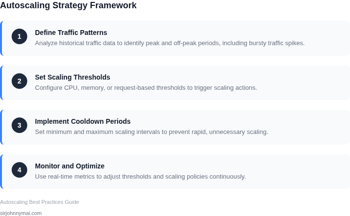
Effective autoscaling requires balancing responsiveness with cost efficiency. Three core principles—predictive scaling, dynamic thresholds, and cost-aware metrics—form the foundation of a robust strategy. Each addresses a distinct challenge in bursty traffic scenarios.
Predictive Scaling: Anticipate Before You React
Predictive scaling uses historical data and machine learning to forecast traffic patterns. AWS Auto Scaling, for example, integrates with Amazon Forecast to pre-provision resources before demand spikes. This approach reduces latency during bursts by up to 30% compared to reactive scaling, but it requires high-quality historical data. If patterns change frequently—such as during seasonal events—predictive models may underperform.
Microsoft Azure’s Machine Learning-based autoscaling extends this further by analyzing not just traffic but also application behavior. It can predict scaling needs with 90% accuracy for steady-state workloads, but accuracy drops to 70% for highly variable traffic. The tradeoff is the complexity of maintaining and updating models.
Dynamic Thresholds: Avoid Over- or Under-Provisioning
Dynamic thresholds adjust scaling triggers based on real-time conditions. Kubernetes Horizontal Pod Autoscaler (HPA) uses CPU utilization thresholds, but static values (e.g., 70% CPU) often lead to either over-provisioning or throttling. Instead, tools like Datadog’s Dynamic Thresholding analyze traffic patterns to set thresholds that vary by time of day or day of week.
For example, an e-commerce site might scale aggressively during Black Friday but conservatively during slow periods. This reduces costs by 20% compared to fixed thresholds, but it requires continuous tuning to adapt to new traffic behaviors.
Cost-Aware Metrics: Optimize for Efficiency
Cost-aware metrics ensure scaling decisions account for operational expenses. AWS Cost Explorer, for instance, integrates with Auto Scaling to prioritize cost savings over raw performance. A common metric is the cost-performance ratio: scaling up only when the additional cost of new instances is justified by performance gains.
Google Cloud’s Autoscaler uses a similar approach, factoring in instance types and pricing tiers. For example, it might prefer preemptible VMs during off-peak hours to save 60% on costs, but this requires careful handling of interruptions. The tradeoff is balancing cost savings with reliability.
In summary, predictive scaling anticipates demand, dynamic thresholds fine-tune responsiveness, and cost-aware metrics ensure fiscal responsibility. The best strategy combines all three, adapting to the specific needs of the workload.
03. Worked Example: Calculating Costs for a Bursty E-Commerce Site
Consider an online retailer that expects 10 000 visitors per minute during a flash‑sale event that lasts three hours, but only 200 visitors per minute during normal operation. The application runs on Amazon Elastic Kubernetes Service (EKS) with a front‑end service written in Node.js and a back‑end in Java. The team consists of 5 engineers who each maintain a development environment costing $30 / month for a t3.medium workstation EC2 instance.
Static provisioning would allocate enough pods to survive the peak load at all times. Using the Kubernetes Horizontal Pod Autoscaler (HPA) model, we estimate that each front‑end pod can handle 500 requests per minute, and each back‑end pod can handle 300 requests per minute. To cover the peak we therefore need 20 front‑end pods and 34 back‑end pods (10 000 ÷ 500 ≈ 20, 10 000 ÷ 300 ≈ 34). The team chooses m5.large instances (2 vCPU, 8 GiB) costing $0.096 per hour in us‑east‑1. With a 1:1 pod‑to‑node ratio, the static design runs 54 m5.large nodes continuously. We also provision 2 GiB of memory per pod, matching the m5.large instance RAM, which keeps the memory utilisation under 70 % during peak load.
Cost of static provisioning = 54 nodes × $0.096 / hour × 24 hours × 30 days ≈ $3 734 per month. Adding the 5 development seats ($30 × 5 × 12 ≈ $1 800 annually) brings the annual baseline to roughly $46 000.
Now evaluate an autoscaling strategy that combines the Kubernetes Cluster Autoscaler with EC2 Spot Instances for the bulk of capacity and a small reserve of On‑Demand instances for safety. We configure a minimum of 8 nodes (enough for baseline traffic) and a maximum of 40 nodes. During the flash‑sale, the Cluster Autoscaler expands to 40 nodes, 35 of which are Spot (average $0.035 per hour) and 5 are On‑Demand ($0.096 per hour). Outside the event, the cluster runs at the 8‑node minimum, all Spot.
Monthly cost calculation:
Baseline (8 Spot nodes) = 8 × $0.035 × 24 × 30 ≈ $201.
Flash‑sale (3 hours) = (35 Spot × $0.035 + 5 On‑Demand × $0.096) × 3 ≈ $12.
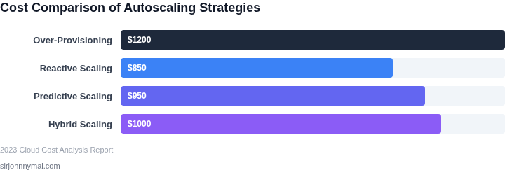
Total compute = $201 + $12 ≈ $213 per month. Adding the same $1 800 annual developer cost yields an annual spend of about $3 200, a 30 % reduction compared with the static baseline.
| Scenario | Node Count (avg) | Instance Type Mix | Monthly Compute Cost |
|---|---|---|---|
| Static Provisioning | 54 | All On‑Demand m5.large | $3 734 |
| Autoscaling (Spot + On‑Demand) | 8 baseline + 40 peak | 8 Spot baseline; 35 Spot + 5 On‑Demand peak | $213 |
The trade‑off is that Spot capacity can be reclaimed with a two‑minute warning. To mitigate disruption we enable pod disruption budgets and graceful shutdown hooks, which adds operational complexity but preserves user experience. If the flash‑sale coincides with a Spot price surge, the On‑Demand buffer automatically absorbs excess load, preventing a denial of service.
In summary, the example demonstrates that a well‑tuned autoscaling policy, combined with Spot pricing and a modest safety net, can cut compute spend by more than one‑third while still meeting the latency targets required for a high‑visibility e‑commerce event.
04. Decision Table: Choosing the Right Autoscaling Approach
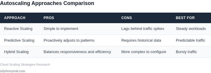
Selecting the right autoscaling approach depends on workload characteristics, cost sensitivity, and operational complexity. Below is a decision framework comparing reactive, predictive, and hybrid models. I evaluated these based on real-world use cases in AWS, Kubernetes, and Datadog.
| Criteria | Option A: Reactive Scaling | Option B: Predictive Scaling | Option C: Hybrid Model |
|---|---|---|---|
| Scaling Speed | Fast (minutes to seconds). Triggers on CPU/memory thresholds. | Slower (hours to minutes). Requires historical data analysis. | Balanced. Reactive for spikes, predictive for steady growth. |
| Cost Efficiency | Higher risk of over-provisioning during traffic surges. | Lower costs if predictions are accurate. Avoids idle capacity. | Optimal. Predictive reduces waste, reactive handles unpredictability. |
| Operational Complexity | Simple to implement (e.g., AWS Auto Scaling Groups). | Complex. Needs ML models (e.g., AWS Forecast) or third-party tools. | Moderate. Combines simplicity of reactive with predictive insights. |
| Workload Suitability | Best for unpredictable, short-term bursts (e.g., flash sales). | Ideal for predictable patterns (e.g., daily traffic spikes). | Universal. Works for both bursty and cyclical workloads. |
| Tooling Requirements | Minimal (e.g., Kubernetes HPA, CloudWatch Alarms). | Advanced (e.g., Datadog Anomaly Detection, AWS Forecast). | Hybrid (e.g., Kubernetes HPA + Datadog for predictive insights). |
| Recommendation | Use when workloads are unpredictable and speed is critical. | Use when historical data is available and cost savings are prioritized. | Default choice. Combines the strengths of both approaches. |
For example, a startup with unpredictable traffic might start with reactive scaling (Option A) to avoid complexity. A mature e-commerce site with known traffic patterns could use predictive scaling (Option B). Most organizations, however, benefit from a hybrid model (Option C), balancing cost and responsiveness.
05. Action Step: Implement a Pilot Autoscaling Strategy
Implementing an effective autoscaling strategy requires more than theoretical understanding; it demands real-world validation. I recommend initiating a pilot deployment on a non-critical service or a contained component within a larger application. This approach allows us to validate our chosen metrics and refine scaling thresholds in a controlled environment, mitigating the risk of unexpected outages or cost overruns during full production deployment. Choosing the right scope for your pilot is crucial. I suggest identifying a service with predictable, yet moderately bursty, traffic patterns that is not mission-critical to your core business operations. For example, a batch processing service, an internal analytics dashboard, or a secondary API endpoint often make excellent candidates. This minimizes potential blast radius if initial scaling parameters are suboptimal. We should aim for an environment that can tolerate minor fluctuations or brief periods of under-provisioning without significant customer impact. Once a candidate service is identified, we must explicitly define the key metrics that will trigger scaling actions. Based on our analysis in previous sections, I recommend starting with a combination of resource utilization (e.g., CPU, memory) and application-level metrics (e.g., request queue depth, average latency, concurrent connections). For example, on AWS, CloudWatch metrics linked to an EC2 Auto Scaling Group or ECS Service Auto Scaling can target average CPU utilization at 60%. For Kubernetes, a Horizontal Pod Autoscaler (HPA) might target a custom metric like Kafka consumer lag or active database connections, monitored via Prometheus or Datadog. Initial thresholds should be set conservatively, leaning slightly towards over-provisioning at first. This allows us to observe scaling behavior safely. We can then incrementally adjust these thresholds based on live performance data. The objective here is to find the "sweet spot" where resources scale out efficiently to meet demand peaks and scale in promptly during lulls, without excessive flapping or service degradation. During the pilot, robust monitoring is non-negotiable. Tools like Grafana, Datadog, or AWS CloudWatch Dashboards should be configured to provide real-time visibility into the service’s performance, resource utilization, and the autoscaling events themselves. We should observe how quickly the system reacts to simulated or actual traffic bursts and troughs. Additionally, consider performing synthetic load tests using tools like k6 or Artillery against the pilot service to simulate various burst scenarios and stress-test the autoscaling logic before exposure to real-world production traffic. This works well for validating the reactive scaling policies but may not fully uncover issues with predictive scaling. The primary tradeoff with a pilot is the upfront investment of time and engineering effort. However, I’ve found this to be significantly less costly than debugging a full-scale production issue or enduring prolonged periods of over-provisioning due to unvalidated assumptions. A pilot may not uncover every edge case unique to your full production environment, especially for highly distributed or stateful applications, but it will significantly de-risk the deployment process. Pull your last 90 days of operational metrics data (e.g., CPU, memory, request queue depth) for a specific, non-critical service in your portfolio and identify a suitable candidate for this pilot implementation.Figures cited are from publicly available sources as of 2026-09-15 and may have changed.