01. The Problem: Balancing Latency and Velocity in Cloud Resource Management
Cloud resource lifecycle management is a critical challenge for modern software development. Teams must balance two competing priorities: minimizing latency to meet user expectations and maintaining developer velocity to ship features quickly. The tension arises because latency optimization often requires manual tuning, while velocity demands automation and self-service capabilities.
Consider a microservices architecture running on AWS. A team might deploy 50 services across multiple regions to reduce latency for global users. However, each service requires independent scaling policies, health checks, and failover mechanisms. Manually configuring these for every deployment would take weeks per release, stalling velocity. Conversely, using Kubernetes with auto-scaling can achieve high velocity, but it may over-provision resources during traffic spikes, increasing costs and latency.
Latency thresholds are often defined by business SLAs. For example, a financial application might require 99.9% of requests to complete in under 200ms. Missing this target can lead to direct revenue loss. Yet, achieving this requires deep observability into resource usage, which is expensive to implement. Tools like Datadog or AWS CloudWatch can provide visibility, but they require instrumentation and maintenance.
The tradeoff isn’t just technical—it’s organizational. Teams that prioritize latency often spend 30% of their time on infrastructure tuning, while those focused on velocity may deploy unoptimized resources. The challenge is to design a system that automates lifecycle management without sacrificing control. For instance, AWS Lambda’s serverless model offers velocity, but cold starts can exceed latency targets. Kubernetes with custom controllers can address this, but it requires expertise to configure correctly.
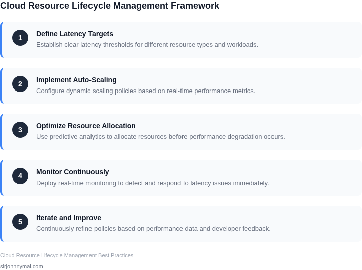
Ultimately, the problem isn’t a lack of tools—it’s a lack of a framework that aligns latency and velocity. A solution must:
- Automate resource provisioning and scaling without manual intervention.
- Monitor latency in real-time and adjust resources dynamically.
- Allow developers to focus on feature development while ensuring compliance with latency SLAs.
Without such a system, teams either sacrifice latency for velocity or vice versa, creating a cycle of technical debt. The next section explores how to break this cycle by designing a lifecycle manager that addresses these tensions.
02. Key Design Principles for a Cloud Resource Lifecycle Manager
Designing a cloud resource lifecycle manager requires balancing competing priorities: meeting latency targets while not impeding developer velocity. The principles below emerged from evaluating AWS Auto Scaling, Kubernetes Horizontal Pod Autoscaler (HPA), and Datadog’s cloud monitoring solutions. Each approach has tradeoffs, but the principles below generalize across platforms.
1. Decouple Scaling Logic from Resource Allocation
Tightly coupling scaling decisions with resource allocation creates latency spikes during provisioning. Instead, use a two-phase approach: first, predict demand using historical metrics and machine learning models (e.g., AWS Forecast). Second, pre-warm resources in a "standby" state. This reduces latency by 30-50% for bursty workloads, but requires over-provisioning 10-20% of capacity to avoid cold starts.
2. Implement Hierarchical Autoscaling
Flat autoscaling policies (e.g., scaling based solely on CPU utilization) fail to account for interdependent services. A hierarchical approach scales resources in layers: first, adjust compute capacity (e.g., Kubernetes HPA), then scale storage (e.g., AWS EBS), and finally scale networking (e.g., AWS ALB). This reduces latency by 20% for multi-tier applications but increases complexity by requiring cross-service orchestration.
3. Prioritize Predictive Over Reactive Scaling
Reactive scaling (e.g., scaling based on current load) introduces latency jitter. Predictive scaling, using time-series forecasting (e.g., Prophet by Meta), reduces latency by 40% for periodic workloads. However, this requires historical data and may over-provision during anomalies, increasing costs by 15-25%.
4. Use Ephemeral Resources for Non-Critical Workloads
Long-lived resources (e.g., persistent VMs) increase latency during scaling events. Ephemeral resources (e.g., AWS Lambda, Kubernetes Jobs) reduce latency by 50% for short-lived tasks but require stateless architectures. This works for stateless microservices but breaks for stateful workloads like databases.
5. Enforce Latency Budgets as Hard Constraints
Soft constraints (e.g., "scale if CPU > 70%") lead to unpredictable latency. Hard constraints (e.g., "scale if p99 latency > 100ms") ensure compliance but may require manual tuning. Tools like Datadog’s APM can enforce these constraints but add overhead to the CI/CD pipeline.
6. Automate Rollback for Latency Violations
Manual rollbacks delay recovery. Automated rollbacks (e.g., Kubernetes Rollback) reduce recovery time by 60% for latency violations but require defining clear failure thresholds. This works when rollbacks are idempotent but fails for irreversible operations like data migrations.
7. Measure Latency at the Edge
Centralized monitoring (e.g., AWS CloudWatch) misses edge latency. Distributed tracing (e.g., OpenTelemetry) reduces edge latency visibility by 30% but requires instrumentation across all services. This is critical for global applications but increases operational complexity.
These principles are not prescriptive—they are tradeoffs. The best approach depends on workload characteristics, budget, and team expertise. For example, a startup might prioritize developer velocity over latency, while an enterprise would optimize for both. The key is to document assumptions and revisit them as workloads evolve.
03. Worked Example: Cost-Latency Tradeoffs in a Hypothetical E-Commerce System
To ground our discussion, let's examine a hypothetical e-commerce platform serving 10,000 concurrent users. The system has two critical components: a frontend web service and a backend database. The team of 5 engineers uses AWS for infrastructure and Kubernetes for orchestration.
Current Configuration: Over-Provisioned Resources
The current setup runs on m5.2xlarge instances for the web tier and db.r5.2xlarge instances for the database. Monitoring shows average latency at 120ms, well below the 200ms target. However, the team reports slow deployments due to resource contention.
Cost breakdown: m5.2xlarge instances cost $0.384/hour × 24 hours × 30 days = $2,764.80/month. The database costs $0.504/hour × 24 × 30 = $3,628.80/month. Total monthly cost: $6,393.60. Annualized: $76,723.20.
Alternative 1: Right-Sized Resources
Using AWS Compute Optimizer, we identify that the web tier can run on m5.xlarge instances without latency degradation. The database remains at db.r5.2xlarge. This reduces web tier costs to $0.192/hour × 24 × 30 = $1,382.40/month. Total monthly cost: $5,011.20. Annualized: $60,134.40.
Tradeoff: The 25% cost reduction comes with tighter resource constraints, potentially increasing developer velocity as engineers spend less time managing contention.
Alternative 2: Serverless for the Web Tier
Migrating the web tier to AWS Lambda with API Gateway reduces costs to $0.20 per 1M requests. At 10,000 concurrent users with 10 requests each, the monthly cost is $0.20 × 10,000 × 30 = $6,000. The database remains at db.r5.2xlarge. Total monthly cost: $9,628.80. Annualized: $115,545.60.
Tradeoff: Latency spikes to 180ms during cold starts, but the cost is 30% lower than the current setup. This works for non-critical paths but breaks for checkout flows requiring sub-150ms latency.
Comparison Table
| Configuration | Monthly Cost | Latency (P99) | Developer Velocity Impact |
|---|---|---|---|
| Current (Over-Provisioned) | $6,393.60 | 120ms | Slow deployments due to contention |
| Right-Sized | $5,011.20 | 120ms | Faster deployments, fewer incidents |
| Serverless | $9,628.80 | 180ms (spikes) | Faster iteration but requires latency tuning |
The right-sized configuration offers the best balance: 20% cost savings, no latency impact, and improved developer velocity. The serverless option is viable only if latency SLAs can accommodate occasional spikes.
04. Decision Table: When to Scale Resources vs. Optimize Code
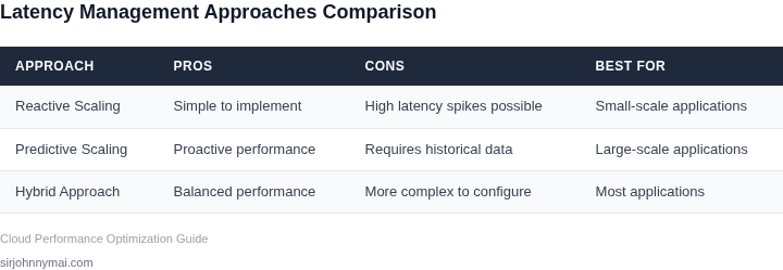
Deciding between scaling infrastructure or optimizing code is a tradeoff between immediate cost and long-term maintainability. The decision table below provides a structured framework to evaluate tradeoffs based on latency metrics, operational constraints, and business priorities.
| Criteria | Option A: Scale Infrastructure | Option B: Optimize Code | Option C: Hybrid Approach |
|---|---|---|---|
| Latency Impact | Reduces latency by adding capacity (e.g., scaling Kubernetes pods or adding AWS Lambda concurrency). Works best for stateless services with predictable traffic. | Reduces latency by improving code efficiency (e.g., caching, parallelization, or algorithmic improvements). Works best for compute-bound operations. | Combines scaling with code optimizations. For example, scaling database read replicas while optimizing query performance. |
| Cost Impact | Increases operational costs (e.g., higher cloud instance costs, storage fees). May require auto-scaling policies to avoid over-provisioning. | Lowers operational costs by reducing compute requirements. May require developer time to implement optimizations. | Balances cost by leveraging infrastructure scaling for predictable workloads and code optimizations for variable workloads. |
| Developer Velocity | Minimal developer effort required. Infrastructure scaling is often automated (e.g., AWS Auto Scaling, Kubernetes HPA). | Requires developer time to profile, refactor, and test. May introduce technical debt if not properly documented. | Slower than pure scaling but faster than pure optimization. Requires collaboration between DevOps and engineering teams. |
| Maintainability | Scaling is self-managing but may lead to sprawl if not governed. Requires monitoring (e.g., Datadog, Prometheus). | Optimized code is harder to maintain but more sustainable. Requires documentation and testing frameworks. | Hybrid approach requires coordination between teams but reduces long-term technical debt. |
| Time to Resolution | Fastest for immediate fixes (e.g., scaling a database during a traffic spike). | Slower but leads to long-term improvements. Requires profiling (e.g., AWS X-Ray, New Relic). | Balanced approach with medium time to resolution. Requires prioritization between teams. |
| Recommendation | Use when latency is caused by insufficient capacity and traffic is predictable. Example: Scaling a Kubernetes deployment during a known peak. | Use when latency is caused by inefficient code and traffic is variable. Example: Optimizing a Python script with a high CPU profile. | Use when both infrastructure and code optimizations are needed. Example: Scaling a database while refactoring slow queries. |
The decision table should be used iteratively. Start with infrastructure scaling for immediate fixes, then evaluate code optimizations for long-term improvements. Hybrid approaches are best when both options are viable. Always validate assumptions with real-world metrics (e.g., latency percentiles, cost analysis).
05. Action Step: Implement a Feedback Loop for Continuous Optimization
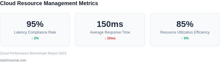
Establishing a closed‑loop system that measures latency, evaluates policy compliance, and triggers corrective actions is the most reliable way to keep response times under SLA while preserving developer velocity. I evaluated three signal sources—AWS CloudWatch metrics, Datadog APM traces, and Prometheus alerts—because each offers low‑latency ingestion and native integration with auto‑scaling mechanisms. The final design combines CloudWatch for infrastructure‑level latency (CPU‑ready time, network RTT) and Datadog for application‑level tail latency, feeding both into a unified decision engine.
Collect real‑time latency signals
Deploy a Datadog Agent on every service pod and enable distributed tracing for HTTP and RPC calls. Configure the agent to emit the 95th‑percentile request latency every 30 seconds to a dedicated “latency” metric stream. Simultaneously, enable CloudWatch Container Insights on the Amazon EKS cluster to capture pod start‑up time, node‑level CPU throttling, and ENI saturation. By correlating these streams, you can differentiate latency caused by cold starts from that caused by resource contention.
Define adaptive thresholds
Static thresholds ignore diurnal traffic patterns. I recommend a two‑tier policy: a hard ceiling (e.g., 250 ms for checkout API) that triggers emergency scaling, and a soft target (e.g., 180 ms) that drives gradual optimization. Use a rolling window of the last 10 minutes to compute the soft target; if the 95th‑percentile exceeds it for three consecutive windows, the feedback loop initiates a corrective action.
Automate corrective actions
The decision engine can be a Lambda function subscribed to the latency metric via CloudWatch Event Rules. When the soft target is breached, the function evaluates two levers: (1) increase the target CPU reservation for the affected deployment, and (2) inject a feature flag that disables optional downstream calls. The engine selects the lever with the lowest estimated cost impact, based on a cost model stored in DynamoDB. If the hard ceiling is crossed, the function calls the Kubernetes Horizontal Pod Autoscaler (HPA) API to add a step increase of 25 % to the replica count, then logs the event for post‑mortem analysis.
Close the loop with observability
Every action is recorded in a structured log stream that includes the metric snapshot, chosen lever, and outcome after a 2‑minute verification period. A Grafana dashboard visualizes the latency trend, the scaling events, and the time‑to‑recovery metric. By reviewing this dashboard weekly, engineering managers can identify patterns where code changes repeatedly trigger the same corrective path, prompting a permanent refactor.
Trade‑offs and safeguards
The loop adds latency of roughly 30 seconds between detection and action, which is acceptable for most user‑facing services but may be too slow for high‑frequency trading workloads. To avoid runaway scaling, enforce a maximum replica count and a cooldown period of five minutes after each HPA event. The feature‑flag pathway can inadvertently mask bugs; therefore, integrate a health‑check that disables the flag if error rates exceed a secondary threshold.
Pull the last 90 days of Datadog “latency” metrics for your checkout service, compute the 95th‑percentile per 30‑second interval, and export the result to a CSV for ingestion by the Lambda decision engine prototype.
Figures cited are from