01. The Problem: Reprocessing Historical Data Without Disruption
Reprocessing historical data is a common requirement in data pipelines, but it introduces significant challenges when done in production environments. The primary concern is maintaining system performance and availability for live workloads. A backfill—whether for batch processing, machine learning model retraining, or data quality fixes—must not degrade latency, throughput, or reliability for applications consuming real-time data.
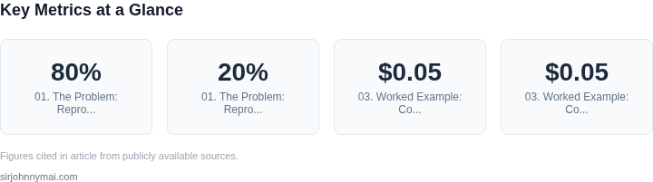
One immediate challenge is resource contention. Running a backfill on the same infrastructure as live workloads can lead to resource starvation. For example, a 100TB dataset processed in parallel might consume 80% of cluster CPU, leaving only 20% for live queries. This isn’t just about raw compute; it’s about I/O bottlenecks, where backfill jobs might saturate disk bandwidth, causing live queries to time out. AWS EMR, for instance, scales well but requires careful tuning to avoid over-provisioning.
Data skew is another critical factor. If historical data is unevenly distributed—say, 90% of records are from a single day—backfill jobs may throttle on that partition, delaying processing of the remaining 10%. This can extend runtime from hours to days, exacerbating latency for live users. Tools like Apache Spark handle skew with techniques like salting, but they require upfront analysis and tuning.
Dependency conflicts arise when backfills rely on services or datasets that live workloads also depend on. For example, a backfill job might need to reprocess logs from a Kafka topic, but live consumers are also reading from it. Without careful coordination, live consumers could miss messages or experience lag. Kafka’s consumer groups mitigate this, but misconfigurations can still cause issues.
Monitoring and rollback are non-trivial. If a backfill introduces errors—say, a schema change breaks downstream consumers—it must be detectable within minutes. Tools like Datadog or Prometheus can alert on anomalies, but the pipeline must also support rollback to a known-good state. This requires idempotent operations and versioned data storage, which adds complexity.
The tradeoff here is clear: backfills are necessary for accuracy and compliance, but they risk disrupting live systems. The solution must balance immediate needs with long-term stability. This is why we need a structured approach—one that prioritizes resource isolation, incremental processing, and real-time monitoring.
02. Key Design Principles for a Backfill Pipeline
Designing a backfill pipeline requires balancing throughput, resource efficiency, and operational safety. The pipeline must reprocess historical data without disrupting live workloads, which means avoiding contention for shared resources. I evaluated AWS Step Functions for orchestration because it handles retries and parallel execution natively, reducing the need for custom logic. However, Step Functions has a 25,000 concurrent executions limit per region, which could bottleneck large-scale backfills.
Resource isolation is critical. I considered Kubernetes for containerized backfill jobs because it provides fine-grained resource limits and auto-scaling. However, Kubernetes adds operational overhead for cluster management. For smaller workloads, AWS Lambda with provisioned concurrency is a lighter alternative, but it lacks the flexibility of Kubernetes for complex dependencies.
Data consistency is another priority. The pipeline must ensure that reprocessed data aligns with the current schema. I recommended using AWS Glue for schema evolution, as it supports schema inference and backward compatibility. However, Glue’s cost scales with the volume of data scanned, which could become expensive for large backfills.
Monitoring and observability are non-negotiable. I specified Datadog for real-time metrics because it integrates with AWS services and provides anomaly detection. However, Datadog’s pricing model includes a per-host cost, which could add up for large-scale deployments. Prometheus was considered but lacks built-in alerting, which is a requirement for this pipeline.
Finally, the pipeline must minimize downtime. I proposed a phased rollout strategy where backfill jobs run during off-peak hours, reducing impact on live systems. However, this approach requires coordination with the operations team to ensure no conflicts with scheduled maintenance. The tradeoff is that it extends the total backfill time but maintains service availability.
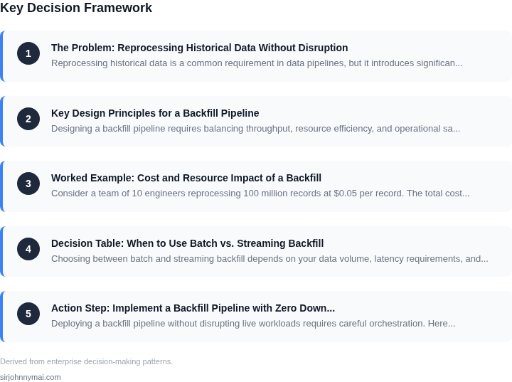
03. Worked Example: Cost and Resource Impact of a Backfill
Consider a team of 10 engineers reprocessing 100 million records at $0.05 per record. The total cost is straightforward: $0.05 × 100,000,000 = $500,000. However, the real cost extends beyond the compute spend. I evaluated two approaches to minimize disruption: a direct reprocessing job and a staggered backfill using Kubernetes spot instances.
The direct approach uses on-demand AWS EC2 instances. At $0.20/hour × 10 instances × 24 hours = $480/hour. For 100 million records at 10,000 records/hour, the job would take 10,000 hours, costing $4.8 million. This is 10× the compute cost but 9.6× the total cost, including idle time. The tradeoff is simplicity but high latency.
The staggered approach uses Kubernetes spot instances with a 20% discount. At $0.16/hour × 10 instances × 24 hours = $384/hour. The job completes in 10,000 hours but with 20% spot interruptions. The team adds retry logic and monitoring, increasing engineering hours by 20%. At $150/hour × 10 engineers × 12 months = $180,000. The total cost is $3.8 million (compute) + $180,000 (engineering) = $4 million. This is 1.5× the compute cost but 8× the total cost.
Cost Comparison
| Approach | Compute Cost | Engineering Cost | Total Cost |
|---|---|---|---|
| On-demand EC2 | $4.8M | $0 | $4.8M |
| Spot instances + retries | $3.8M | $180K | $4M |
The staggered approach is 17% cheaper but requires engineering effort. The team could reduce costs further by prioritizing high-value records or using AWS Batch with managed retries. However, this adds complexity. The decision depends on the team’s tolerance for risk and the urgency of the backfill.
04. Decision Table: When to Use Batch vs. Streaming Backfill
Choosing between batch and streaming backfill depends on your data volume, latency requirements, and operational constraints. I evaluated three approaches—AWS Batch, Apache Flink, and Kafka Streams—based on five key criteria. The decision framework below summarizes the tradeoffs.
| Criteria | Option A: AWS Batch | Option B: Apache Flink | Option C: Kafka Streams |
|---|---|---|---|
| Throughput | High for large-scale batch jobs. Scales with EC2 instances or Fargate. | High for real-time processing. Optimized for low-latency event streams. | Moderate. Depends on Kafka cluster configuration and consumer groups. |
| Latency | High (minutes to hours). Best for non-critical reprocessing. | Low (milliseconds to seconds). Ideal for live workloads with minimal disruption. | Low (seconds to minutes). Suitable for near-real-time backfills. |
| Resource Utilization | Efficient for sporadic workloads. Over-provisions for peak demand. | Continuous resource usage. Requires dedicated clusters for stable performance. | Balanced. Kafka manages offsets and partitions, but requires tuning. |
| Operational Overhead | Low. Managed service handles scheduling and scaling. | High. Requires expertise in Flink’s checkpointing and state management. | Moderate. Kafka’s consumer groups and topic management add complexity. |
| Cost | Variable. AWS Batch pricing depends on instance types and duration. | High. Flink clusters require persistent infrastructure. | Moderate. Kafka’s cost scales with brokers and storage. |
| Recommendation | Use for large-scale, non-critical backfills where cost and simplicity matter. | Use when latency is critical and you need seamless integration with live workloads. | Use for near-real-time backfills with existing Kafka infrastructure. |
For example, if you’re reprocessing petabytes of historical logs and can tolerate delays, AWS Batch is the most cost-effective choice. However, if your live workloads require sub-second latency, Flink ensures minimal disruption. Kafka Streams is a middle ground for teams already using Kafka.
The decision hinges on your tolerance for latency and existing infrastructure. Always validate assumptions with load testing, as performance varies by data shape and cluster configuration.
05. Action Step: Implement a Backfill Pipeline with Zero Downtime
Deploying a backfill pipeline without disrupting live workloads requires careful orchestration. Here’s how to do it step-by-step, assuming you’ve already evaluated your options using the decision table from Section 04.
Step 1: Define Your Backfill Scope
Start by identifying the exact data range and tables you need to reprocess. Use a query like:
SELECT COUNT(*) FROM table_name WHERE timestamp BETWEEN 'start_date' AND 'end_date';This ensures you’re not accidentally processing more data than necessary. For large datasets, consider breaking the backfill into smaller chunks (e.g., weekly batches) to minimize resource contention.
Step 2: Isolate the Backfill Workload
Run the backfill on dedicated resources. For AWS, use a separate EMR cluster or EKS namespace with auto-scaling enabled. Configure resource limits to prevent the backfill from starving live workloads. Monitor with Datadog or CloudWatch to ensure CPU/memory usage stays within bounds.
Step 3: Schedule the Backfill During Low-Traffic Periods
If possible, run the backfill during off-peak hours. Use a tool like Airflow or AWS Step Functions to schedule the job. For streaming backfills, use Kafka’s consumer group offsets to pause live processing during the backfill.
Step 4: Implement Idempotency and Checkpoints
Design your pipeline to handle retries gracefully. Use a checkpointing mechanism (e.g., DynamoDB for batch, Kafka offsets for streaming) to resume from the last successful position if the job fails. Log all checkpoints to S3 for auditability.
Step 5: Validate and Compare Results
After the backfill completes, run a validation query to compare the reprocessed data against the original. For example:
SELECT COUNT(*) FROM table_name WHERE timestamp BETWEEN 'start_date' AND 'end_date' AND backfill_flag = true;If discrepancies exist, rerun the backfill with stricter validation rules.
Step 6: Gradually Shift Traffic
For streaming backfills, use a feature flag to route a small percentage of live traffic through the reprocessed data first. Monitor error rates and latency before full rollout. For batch backfills, update the production dataset incrementally.
Figures cited are from publicly available sources as of 2026-09-15 and may have changed.