How to build a machine learning feature store that your team will actually use

The Silent Failure of Feature Stores

Most machine learning feature store initiatives fail not because of engineering incompetence, but because of an adoption mismatch. Organizations routinely invest hundreds of thousands of dollars building or licensing high-performance feature stores, only to find their data science teams bypassing them entirely. These teams continue to write bespoke, siloed SQL queries and Pandas pipelines for training, while engineering struggles to reconstruct those same features in low-latency production APIs.

The core issue is that platform engineering teams often treat a feature store as a database infrastructure problem. In reality, it is a product management challenge. If your feature store adds friction to the data scientist's inner loop—the rapid iteration between hypothesis, data preparation, and model evaluation—it will be rejected. To build a system that teams actually use, you must balance developer ergonomics, point-in-time correctness, and low-latency serving. This guide outlines how we approach this architectural and organizational challenge at scale.

01. The User-Empathy Gap in MLOps

To design a successful feature store, you must understand the conflicting incentives of its two primary users: the Data Scientist (DS) and the Software/Production Engineer (SWE). These two personas have fundamentally different requirements for their development environments and runtime systems.

The Data Scientist operates in a world of high throughput and offline analysis. They care about expressiveness, Python compatibility, historical completeness, and fast iteration. Their metric of success is model accuracy (e.g., AUC, F1-score). If a feature store forces them to write complex Java/Scala wrappers or wait hours for a batch pipeline to register a new feature, they will revert to local CSV exports and custom preprocessing scripts.

The Software Engineer operates in a world of low latency, high availability, and deterministic behavior. They care about 99th-percentile (p99) latency, write-safety, monitoring, and horizontal scaling. Their metrics are system-level: CPU utilization, memory footprints, and request-per-second (RPS) limits. They do not care about the mathematical elegance of a feature; they care if evaluating that feature breaches their 50-millisecond SLA.

A feature store must act as a translator between these two worlds. It must provide a simple Python SDK for the Data Scientist to define and pull historical data, while automatically compiling those definitions into highly optimized, low-latency key-value lookups for production systems. If your architecture forces either party to compromise their core metrics, the platform will face critical adoption hurdles.

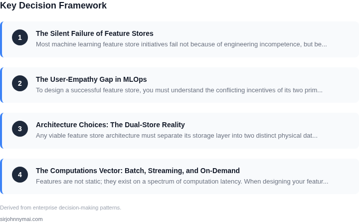
02. Architecture Choices: The Dual-Store Reality

Any viable feature store architecture must separate its storage layer into two distinct physical databases: an Offline Store and an Online Store. This is known as the dual-store pattern. Attempting to run both workloads on a single database engine guarantees failure, as analytical queries will starve production transactional reads of system resources.

The Offline Store handles high-throughput, historical data. It is optimized for large-scale batch queries, such as generating training datasets spanning millions of rows and hundreds of features. The underlying technology is typically an analytical column-store database or data lakehouse, such as Snowflake, Google BigQuery, Amazon S3 (using Apache Parquet format), or Databricks (using Delta Lake). The key metric here is throughput per dollar and query expressivity.

The Online Store handles low-latency, single-record lookups. It is populated by materialization pipelines that sync data from the offline store or stream ingest pipelines directly. The underlying technology must be an in-memory or highly optimized NoSQL database, such as Redis, Amazon DynamoDB, or Cassandra. The key metric here is p99 read latency, which must typically remain under 10 milliseconds.

The fundamental challenge of the dual-store architecture is skew. Skew occurs when the logic used to compute features for the offline store differs from the logic used to compute or retrieve features for the online store. This discrepancy leads to training-serving skew, where a model performs exceptionally well in offline validation but fails catastrophically in production because the feature values do not match.

---

03. The Computations Vector: Batch, Streaming, and On-Demand

Features are not static; they exist on a spectrum of computation latency. When designing your feature store, you must explicitly categorize features into three computational vectors based on how frequently the underlying data changes and how quickly those changes must reflect in production models.

Batch Features: These are features computed on a regular schedule (e.g., nightly, hourly) using large-scale processing engines like Apache Spark, dbt, or Snowflake SQL. Examples include "average transaction value over the past 30 days" or "user category affinity." These features are written to the offline store first, then materialized to the online store on a schedule. This pattern is highly cost-effective and simple to manage, but it cannot capture real-time behavioral changes.

Streaming Features: These are features computed continuously over real-time event streams (e.g., Apache Kafka, Amazon Kinesis) using stream processing engines like Apache Flink or Spark Streaming. Examples include "number of login attempts in the last 5 minutes." These features are written directly to the online store to ensure sub-second freshness, while a parallel process writes them to the offline store for future training runs.

On-Demand (Real-Time) Features: These are features that cannot be pre-computed because they rely on data only available at the exact moment of the prediction request. Examples include "distance between current transaction location and user's home address" or "current shopping cart value combined with real-time weather data." These features must be computed inline within the model serving container or by a lightweight microservice at query time.

Concrete Worked Example: Financial Transaction Fraud Feature

Let us analyze the engineering trade-offs and physical costs of implementing a feature called user_velocity_score (the number of transactions a user has completed in the last 10 minutes) across 10 million active users. We will compare two approaches: Batch Pre-computation with Redis materialization vs. On-Demand Calculation with DynamoDB raw state lookups.

Option A: Batch Pre-computation in Redis

In this scenario, we compute the transaction count for all 10 million active users every 10 minutes using an Apache Spark job, then write the results to a Redis cache for sub-millisecond production retrieval.

• Data Size: Each user record consists of a 64-bit integer user ID (8 bytes) and a 32-bit integer transaction count (4 bytes). Total raw payload per user = 12 bytes.
• Redis Memory Overhead: Redis data structures introduce significant metadata overhead (approx. 250 bytes per key-value pair under standard Redis configuration). Total physical memory required per user record: ~262 bytes.
• Total RAM Requirement: 10,000,000 users * 262 bytes = 2,620,000,000 bytes (~2.44 GiB).
• Infrastructure Requirements: To support high availability and p99 read SLAs under high query volume, we deploy an Amazon ElastiCache for Redis cluster with 1 primary node and 1 read replica. We select the cache.m6g.large instance class (6.38 GiB RAM, up to 10 Gbps network bandwidth).
• Cost Calculation: The cost of a cache.m6g.large instance is approximately $0.132 per hour. Running 2 nodes (1 primary, 1 replica) for 730 hours per month yields:

  2 nodes * $0.132/hour * 730 hours = $192.72 per month

• Latency Profile: Redis read latency (p99) is consistently under 2 milliseconds. However, the data latency (freshness) is bounded by the 10-minute Spark run interval. A transaction occurring 1 minute after the last run is invisible to the model for another 9 minutes.

Option B: On-Demand Calculation with DynamoDB and AWS Lambda

To achieve absolute real-time accuracy, we do not pre-compute the count. Instead, we write every raw transaction event to Amazon DynamoDB with a Time-To-Live (TTL) set to 10 minutes. When a prediction request arrives, an AWS Lambda function queries DynamoDB for all transaction records for that user in the last 10 minutes and computes the count on the fly.

• DynamoDB Write Throughput: Assuming an average of 500 new transactions per second globally across the user base. Each transaction write requires 1 Write Capacity Unit (WCU).
• DynamoDB Read Throughput: The model is evaluated 1,000 times per second. Each evaluation requires querying the last 10 minutes of transactions for a specific user. Assuming a user averages 1.2 transactions in a 10-minute window, this query returns ~1.2 records, which fits comfortably within a single strongly consistent Read Capacity Unit (RCU). Total required RCUs = 1,000 per second.
• Infrastructure Costs:
  • DynamoDB Provisioned Capacity: 500 WCUs ($0.00065 per WCU-hour) and 1,000 RCUs ($0.00013 per RCU-hour):

    (500 * $0.00065 * 730) + (1,000 * $0.00013 * 730) = $237.25 + $94.90 = $332.15 per month

  • AWS Lambda Compute Cost: 1,000 invocations per second = 2.59 billion invocations per month. Assuming an average execution time of 15ms on a 512MB Lambda function ($0.0000000083 per 1ms):

    2.592B * 15ms * $0.0000000083 = $322.70 per month

  • Total Monthly Cost: $332.15 (DynamoDB) + $322.70 (Lambda) = $654.85 per month
• Latency Profile: DynamoDB query latency (p99) is approximately 12ms. Lambda execution adds 15ms of compute latency. Network serialization adds another 8ms. Total p99 latency for on-demand generation is approximately 3