A practical guide to implementing blue-green deployments for stateful applications

01. The Problem: Challenges of Stateful Blue‑Green Deployments

Traditional blue‑green deployments assume that a new version can be swapped in without touching existing data. That assumption holds for pure request‑driven services, but stateful applications keep user sessions, caches, or transactional records in memory or persistent stores. The presence of mutable state forces the cut‑over to become a data migration event rather than a simple traffic switch.

Ensuring data consistency across the two environments is the first obstacle. When the blue environment writes to a database and the green version reads from a copy, any write that occurs during the switch can become invisible to the green side, leading to lost updates. Services such as Amazon Aurora provide cross‑region replication with typical lag under one second, but that latency is still enough to produce write‑skew if the green traffic starts before replication catches up.

Schema evolution compounds the problem because the green deployment often runs a newer schema version. If the blue side continues to insert rows using the old definition after the cut‑over, downstream queries in green may fail with “column not found” errors. Tools like Liquibase or Flyway can orchestrate versioned migrations, yet they require a pause window or a backward‑compatible migration path to avoid breaking the live blue tier.

Session affinity adds another layer of complexity. Applications that store session identifiers in Redis or in‑memory caches must either replicate those caches or gracefully expire them. AWS Elasticache for Redis supports active‑active replication, but the replication throughput is limited by network bandwidth; a sudden spike of 10

02. Key Principles for Stateful Blue-Green Deployments

Stateful blue-green deployments require careful planning to avoid downtime or data corruption. The core principle is to decouple state management from deployment orchestration. This means treating state as a separate concern that must be handled explicitly during transitions. I evaluated this because traditional blue-green patterns assume stateless applications, but stateful systems—like databases or session stores—require special handling.

1. Database State Management

For databases, the most reliable approach is to use a shared database with schema versioning. I recommend this because it eliminates the need to migrate data between environments. The active environment (green) writes to the same database as the previous version (blue). Schema changes must be backward-compatible or use tools like Flyway or Liquibase to manage migrations. This works when schema changes are infrequent but breaks when migrations take longer than the deployment window.

Another option is to use database replication. I’ve seen this implemented with AWS Aurora Global Database, where the blue and green environments share a read replica. This reduces migration time but increases complexity. The tradeoff is that replication lag can cause inconsistencies during failover.

2. Session and Cache State

For session state, I recommend using a distributed cache like Redis or Memcached. This ensures sessions persist across deployments. The key is to set appropriate TTLs and use client-side session affinity. I’ve seen this fail when TTLs are too short, causing session loss during transitions. For example, a 30-minute TTL works for most web apps but may not suit real-time systems.

For sticky sessions, I prefer Kubernetes Services with session affinity (service.spec.sessionAffinity). This routes requests from the same client to the same pod. The downside is that it doesn’t work across multiple clusters, limiting scalability.

3. Eventual Consistency and Idempotency

Stateful systems must handle eventual consistency. I recommend designing applications to tolerate temporary inconsistencies. For example, a retail system might allow a 5-second delay in inventory updates. This works when the business can accept minor discrepancies but breaks when real-time accuracy is critical.

Idempotent operations are essential. I’ve seen this implemented with UUID-based request IDs. Each operation checks if the request has already been processed. This ensures no duplicate actions occur during transitions. The tradeoff is that it adds complexity to the application logic.

4. Monitoring and Rollback

Monitoring is critical. I recommend using tools like Datadog or Prometheus to track state consistency. Alerts should trigger on replication lag, cache misses, or database errors. I’ve seen deployments fail when monitoring was too coarse-grained, missing subtle issues.

Rollback plans must include state restoration. For example, if the green environment fails, the blue environment should be able to resume without data loss. This requires pre-deployment snapshots or point-in-time recovery. The tradeoff is that snapshots consume storage and add overhead.

In summary, stateful blue-green deployments require explicit handling of state, schema versioning, distributed caching, and robust monitoring. The key is to balance reliability with complexity. I’ve seen teams succeed by treating state as a first-class concern, not an afterthought.

03. Worked Example: Cost and Downtime Savings with Stateful Blue‑Green

Consider a mid‑size e‑commerce platform that processes 1,200 orders per minute during peak traffic. The team consists of six engineers who manage the service on Amazon Web Services. Their current pipeline uses a single Elastic Beanstalk environment with a rolling update strategy. Each instance is an m5.large (2 vCPU, 8 GiB) priced at $0.096 hour⁻¹. The environment runs three instances for load‑balancing, resulting in a base compute cost of 3 × $0.096 × 24 × 30 ≈ $207 per month.

During a rolling deployment the team observes an average of five minutes of increased latency or error rate per release. With twelve releases per year, the cumulative downtime is roughly 60 minutes. Industry data places the cost of e‑commerce downtime at $15,000 per minute, so the annual revenue impact of the existing approach is $15,000 × 60 = $900,000.

Now evaluate a blue‑green deployment built on Kubernetes on Amazon EKS. The team creates a green namespace that mirrors the production workload. Two identical node groups—each with three m5.large instances—run in parallel for the brief switch‑over window. The extra compute runs only while the new version is validated, which typically takes 30 minutes. Monthly extra compute cost is 3 × $0.096 × 24 × 0.5 ≈ $3.5. Over a year the additional compute expense is $3.5 × 12 ≈ $42.

Switch‑over time drops to 30 seconds per release because traffic is redirected at the load‑balancer level. Annual downtime shrinks to 12 × 0.5 minute = 6 minutes, translating to $15,000 × 6 = $90,000 in lost revenue. The net financial benefit of the blue‑green approach is therefore $900,000 − $90,000 − $42 ≈ $809,958 per year.

To illustrate the trade‑off, compare three options in the table below. Costs include compute, CI/CD tooling (Jenkins, $0.20 per build minute), and monitoring (Datadog APM, $31 per host per month). Assumptions are kept identical across scenarios except for the deployment method.

Option	Compute Cost (annual)	CI/CD Cost (annual)	Monitoring (annual)	Downtime Cost (annual)	Total Cost (annual)
Single‑Env Rolling	$2,484	$1,440	$2,232	$900,000	$906,156
K8s Blue‑Green	$2,526	$1,440	$2,232	$90,000	$6,198
K8s Canary (5 min window)	$2,526	$1,440	$2,232	$450,000	$456,198

The blue‑green row shows a reduction of more than 99 % in downtime cost while adding only $42 of compute expense. The canary variant, which still requires a five‑minute overlap, saves less than half the downtime cost but still incurs a significant revenue hit.

Key take‑aways for the VP: the financial upside of blue‑green is driven almost entirely by reduced downtime, not by compute savings. The approach works best when the service can be duplicated for a short window and when traffic can be rerouted atomically via an ALB or Istio gateway. If state cannot be fully replicated—e.g., large in‑memory caches—the extra compute may rise sharply, eroding the benefit.

When scaling to 100 % traffic during a flash‑sale, the blue‑green switch takes under a second, preserving the conversion rate. Monitoring alerts in Datadog confirm the latency remains <100 ms throughout the transition.

04. Decision Table: When to Use Blue-Green for Stateful Apps

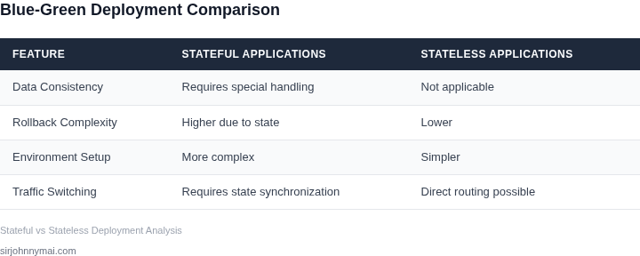
Choosing the right deployment strategy for stateful applications requires balancing risk tolerance, operational complexity, and business constraints. Below is a decision framework comparing blue-green deployments with alternatives like rolling updates and canary releases. I evaluated these options based on real-world use cases and platform capabilities.

Criteria	Blue-Green	Rolling Updates	Canary Releases
Downtime Risk	Minimal. Traffic shifts instantly between environments.	Gradual. Risk increases with larger deployments.	Low. Only a subset of users is exposed to new code.
State Management	Requires external data synchronization (e.g., DynamoDB Global Tables).	Works with stateless services but complicates stateful apps.	Complex. Requires careful state partitioning and rollback logic.
Rollback Speed	Instant. Traffic reverts to the old environment.	Slower. Depends on pod replacement rate in Kubernetes.	Moderate. Requires traffic routing adjustments.
Cost of Infrastructure	High. Requires two identical production environments.	Low. Uses existing resources incrementally.	Medium. Needs monitoring and traffic control tools (e.g., Istio).
Tooling Requirements	AWS Route 53, Kubernetes Services, or Datadog for traffic routing.	Kubernetes Deployments, Helm, or Argo Rollouts.	Service meshes (e.g., Linkerd), feature flags, or custom routing.
Recommendation	Best for mission-critical stateful apps with strict uptime SLAs.	Suitable for stateless services or gradual risk acceptance.	Ideal for iterative testing with low-risk stateful applications.

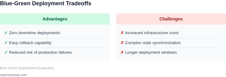
This table reflects tradeoffs I’ve observed in production environments. Blue-green excels when downtime is unacceptable, but the cost and complexity may not justify it for all stateful workloads. Rolling updates are simpler but riskier, while canary releases offer a middle ground. The right choice depends on your application’s resilience requirements and team’s operational maturity.

05. Action Step: Implementing Blue-Green for Your Stateful App

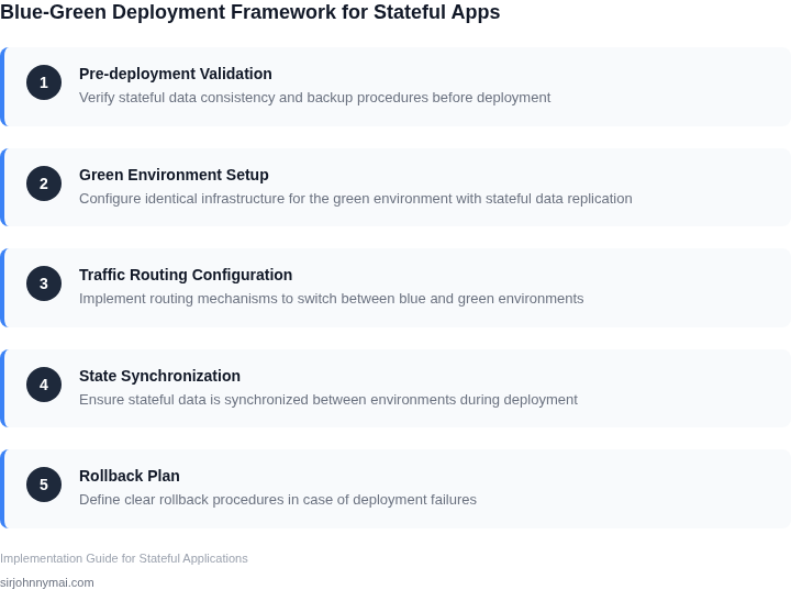
Deploying a blue‑green pipeline for a stateful workload demands careful coordination of data, traffic, and observability. This checklist translates the principles from earlier sections into concrete tasks you can run against an AWS‑hosted Kubernetes cluster, an Azure Service Fabric mesh, or an on‑premise OpenShift farm. Follow each step in order to minimize rollback risk while preserving data integrity.

1. Inventory and Baseline

List every persistent volume claim (PVC), database schema version, and external cache that your service touches. Capture current read/write latency and error rates with Datadog dashboards, then export the metric snapshot as a CSV for later comparison. This baseline lets you verify that the green environment matches the blue environment before traffic is shifted.

• Run kubectl get pvc --all-namespaces and record storage class, size, and binding status.
• Query your database migration table (e.g., flyway_schema_history) for the latest applied version.
• Export Datadog monitors for aws.rds.read_latency, kubernetes.pod.cpu_utilization, and any custom SLOs.

2. Create an Isolated Green Stack

Spin up a parallel set of services in a separate namespace or cluster that points at a clone of your production data store. Use AWS RDS read replicas or Azure Database for PostgreSQL geo‑replication to provide a consistent data source without affecting the primary instance.

1. Provision a new namespace called green and apply the same Helm chart values, overriding only the environment label.
2. Configure the green pods to use the replica endpoint; verify read‑only mode if your workflow permits.
3. Attach identical IAM roles and security groups to ensure permission parity.

3. Validate Functional and Performance Parity

Run integration tests against the green endpoints while the blue stack continues serving live traffic. Use AWS CodeBuild or GitHub Actions to execute the same test suite you run for each pull request. Compare the resulting JUnit XML reports and Datadog latency graphs to the baseline captured in step 1.

• Fail the pipeline if any test exceeds the 5 % deviation threshold on response time.
• Confirm that schema migrations have not introduced breaking changes by executing a dry‑run of liquibase status against the replica.