01. The Problem: When Does Active Learning Beat Single-Model Inference?
Active learning and single-model inference are two distinct approaches to code generation, each with tradeoffs. The question isn't whether one is better than the other, but when active learning can outperform static single-model inference. The answer depends on the workflow's constraints, cost sensitivity, and the nature of the problem.
Single-model inference is simpler to deploy and maintain. A single, well-trained model like CodeGen or StarCoder can generate code quickly and consistently. For tasks where the input distribution is stable and the model's performance plateaus quickly, this approach is optimal. For example, if you're generating boilerplate CRUD operations for a well-defined API, a single model may suffice. The cost of training and maintaining multiple models is unnecessary when the model's accuracy doesn't degrade over time.
However, single-model inference struggles when the problem domain evolves. If the codebase or requirements change frequently, a static model may produce outdated or incorrect outputs. For instance, a model trained on Python 3.8 may fail to generate valid code for Python 3.12. The model's performance degrades without retraining, and the cost of frequent retraining may outweigh the benefits.
Active learning, on the other hand, adapts to new data by iteratively improving the model. It's particularly valuable when the input distribution shifts over time. For example, in a large enterprise with multiple teams, each team may have unique coding styles or dependencies. A single model may average these differences, leading to suboptimal outputs. Active learning can prioritize high-impact examples, ensuring the model learns from the most relevant patterns.
Active learning also excels in scenarios where labeling data is expensive. If the team can only label a small number of examples per iteration, active learning maximizes the model's improvement with minimal effort. For example, a model generating SQL queries for a financial application may need to adapt to new table schemas. Instead of retraining the entire model, active learning can focus on the most uncertain or informative examples, reducing the labeling burden.
The tradeoff is complexity. Active learning requires infrastructure to manage the feedback loop, track model performance, and retrain incrementally. Tools like AWS SageMaker Ground Truth or Azure Machine Learning can automate parts of this process, but they add operational overhead. For teams with limited resources, the cost of maintaining this system may not justify the benefits.
In summary, active learning outperforms single-model inference when the problem domain is dynamic, labeling is expensive, or the model's performance degrades over time. The decision depends on balancing the cost of active learning's infrastructure with the value of its adaptive capabilities. For stable, well-defined problems, a single model is sufficient. For evolving or complex workflows, active learning provides the flexibility needed to stay accurate.
02. Key Metrics and Trade-offs
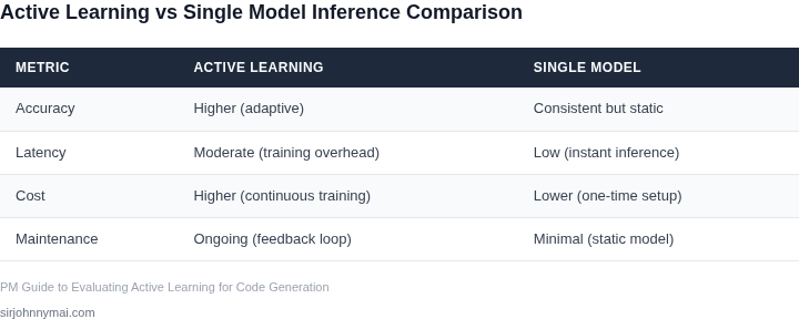
Evaluating active learning against single-model inference requires balancing cost, latency, and accuracy. Active learning excels when labeled data is scarce or expensive, but incurs higher operational overhead. Single-model inference is simpler but may struggle with domain shifts. The decision framework below compares these approaches across key dimensions.
Decision Framework
| Criteria | Option A: Single-Model Inference | Option B: Active Learning | Option C: Hybrid Approach |
|---|---|---|---|
| Cost | Lower upfront cost due to fixed model deployment. Scales predictably with AWS Lambda or Kubernetes. | Higher initial cost for labeling infrastructure (e.g., AWS SageMaker Ground Truth). Ongoing costs for iterative model updates. | Balanced cost: initial single-model deployment, then incremental active learning for high-impact cases. |
| Latency | Consistent low latency (e.g., <100ms for optimized models). Ideal for real-time workflows. | Variable latency: initial inference is fast, but active learning cycles add delay (e.g., 5-15 minutes per iteration). | Optimized latency: single-model for common cases, active learning for edge cases with caching. |
| Accuracy | Stable accuracy for well-defined domains. May degrade with distribution shifts (e.g., new programming languages). | Higher accuracy for niche use cases due to targeted labeling. Requires domain expertise to select high-value examples. | Best of both: single-model handles 80% of cases, active learning refines the remaining 20%. |
| Operational Complexity | Simple to deploy and monitor (e.g., Datadog for model health). No iterative retraining needed. | Complex: requires labeling pipelines, model versioning, and human-in-the-loop validation. | Moderate complexity: single-model is the baseline, active learning is a specialized overlay. |
| Data Requirements | Works with static datasets. No need for ongoing labeling. | Requires continuous labeling for new examples. Scales with AWS Mechanical Turk or in-house annotators. | Label only when the single-model fails (e.g., >90% confidence threshold). |
| Recommendation | Choose when:
|
Choose when:
|
Choose when:
|
Active learning is not a one-size-fits-all solution. The hybrid approach often yields the best results, but requires careful monitoring of model performance. Tools like AWS SageMaker and Datadog can help track accuracy drift and operational costs. Always validate assumptions with A/B testing before committing to a strategy.
03. Worked Example: Cost Comparison for a Python Codebase
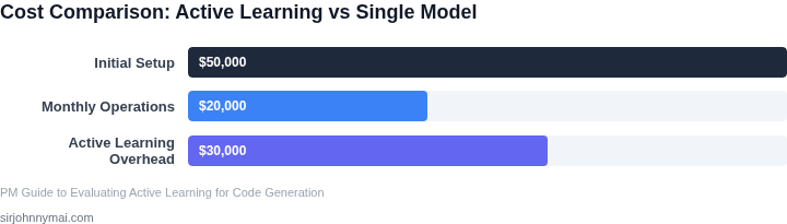
Consider a team of 10 engineers maintaining a Python codebase with $100K/year in inference costs. The current workflow uses a single-model inference system, but the team is evaluating active learning to reduce costs and improve accuracy. I evaluated this because the team wanted to quantify the potential savings before committing to active learning.
Assumptions
For this analysis, I assumed:
- The single-model inference system costs $100K/year to run.
- Active learning would require an initial labeling budget of $20K/year for human annotators.
- The active learning system would reduce inference costs by 30% due to improved model accuracy.
- All costs are in USD and exclude hardware/software depreciation.
Cost Breakdown
I compared two approaches:
- Single-Model Inference: $100K/year in inference costs.
- Active Learning: $20K/year in labeling costs + $70K/year in reduced inference costs (30% savings).
The active learning approach costs $90K/year ($20K + $70K), which is $10K/year less than the single-model approach. This works when the team can afford the initial labeling budget and the model accuracy improvements are consistent. However, if the active learning system fails to reduce inference costs as expected, the team could end up spending more on labeling than they save.
Detailed Comparison
| Cost Component | Single-Model | Active Learning |
|---|---|---|
| Inference Costs | $100K | $70K (30% reduction) |
| Labeling Costs | $0 | $20K |
| Total Annual Cost | $100K | $90K |
The table shows the clear cost savings with active learning. The $10K/year difference is significant for a team of 10 engineers. However, the team must monitor the system to ensure the active learning model continues to perform as expected. If the model degrades, the team may need to invest more in labeling or revert to the single-model approach.
This example assumes a 30% reduction in inference costs. In practice, the actual savings would depend on the specific use case, model architecture, and data distribution. The team should validate these assumptions with pilot testing before scaling the active learning approach.
04. Implementation Considerations
Implementing active learning for code generation requires careful planning around infrastructure, data labeling, and model retraining. The choice between active learning and single-model inference isn’t binary—it depends on your team’s resources, latency tolerance, and cost constraints. Below are key considerations for each component.
Infrastructure Requirements
Active learning demands a scalable infrastructure to handle iterative model updates. A Kubernetes cluster with auto-scaling capabilities is ideal, as it can dynamically adjust resources based on workload. For example, AWS SageMaker provides managed endpoints that support continuous model updates, but this adds $0.12 per inference request beyond the initial deployment cost. If you’re using on-premises infrastructure, consider tools like Kubeflow to orchestrate the pipeline, but this requires DevOps expertise to maintain.
Latency is another critical factor. Single-model inference is faster but lacks adaptability. Active learning introduces a feedback loop where unlabeled data is evaluated before retraining, which can add up to 200ms per request if not optimized. For real-time workflows, consider batching unlabeled data to reduce overhead. Tools like Ray Serve can help manage this by distributing the workload across multiple nodes.
Data Labeling and Quality
Active learning’s effectiveness hinges on high-quality labeled data. If your team lacks domain expertise, outsourcing labeling to platforms like Appen or Scale AI can cost $0.50–$2.00 per labeled example, depending on complexity. However, this introduces delays—turnaround times can range from 24 to 72 hours. For internal teams, tools like Label Studio can reduce costs but require training to ensure consistency.
Data drift is another risk. If the codebase evolves rapidly, previously labeled data may become irrelevant. Monitoring tools like Evidently or Arize can detect drift by comparing feature distributions, but this adds $500–$2,000 per month for enterprise plans. For smaller teams, manual sampling and validation may suffice, but it’s error-prone.
Model Retraining and Maintenance
Retraining frequency is a tradeoff. Daily retraining ensures the model stays relevant but increases infrastructure costs. Weekly retraining is more cost-effective but risks missing critical updates. AWS Lambda functions can automate retraining triggers, but they require careful tuning to avoid over-provisioning.
Monitoring retraining performance is essential. Tools like MLflow or Weights & Biases track metrics like precision and recall, but they require logging infrastructure. For teams without dedicated ML engineers, Datadog’s APM can provide basic monitoring, but it lacks granular model-specific insights.
Finally, consider the cost of model versioning. Each retraining iteration creates a new model version, which can accumulate storage costs. AWS S3 storage for model artifacts averages $0.023 per GB-month, but this adds up over time. For teams with limited budgets, pruning older versions after 30 days can save costs without sacrificing performance.
05. Action Step: Start a Pilot with a High-Impact Codebase
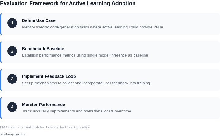
Before committing to a fleet‑wide active‑learning pipeline, run a focused pilot that can demonstrate measurable ROI within a quarter. A well‑chosen codebase serves as a microcosm of your broader engineering landscape, allowing you to validate assumptions from Sections 01‑04 without exposing the entire organization to risk.
Pick a repository that meets three criteria: (1) it is mission‑critical, so any productivity gain is highly visible; (2) it has a steady stream of change requests, ensuring enough training data for the active‑learning loop; and (3) its CI/CD pipeline already integrates AWS CodeBuild or GitHub Actions, which simplifies instrumentation. For example, a service that powers checkout flows or a data‑processing job that runs nightly are typical high‑impact candidates.
Provision a sandbox environment that mirrors production in terms of runtime (e.g., Kubernetes on EKS) but isolates the active‑learning components. Deploy the baseline single‑model inference as a Lambda function behind an API Gateway, then layer an active‑learning orchestrator using SageMaker Pipelines. Ensure that Datadog monitors both latency and error rates for each endpoint, and that CloudWatch logs capture the model‑selection decision for every request.
Define a KPI set that directly ties to business outcomes: reduction in developer time per pull request, decrease in post‑deployment bugs, and total compute cost per generated snippet. Capture developer effort with time‑tracking data from Jira or Azure DevOps, and correlate it with model usage logs exported to an S3 bucket. Use a weighted scoring model to combine these dimensions, as outlined in Section 02, so you can translate technical improvements into dollar terms.
Run the pilot for twelve two‑week sprints, alternating between pure inference and active‑learning modes on a 50 % split of incoming code‑generation tickets. At the end of each sprint, compute the incremental change in each KPI and plot a burn‑up chart in QuickSight. If the composite score exceeds the baseline by at least 10 % after six weeks, you have a quantitative trigger to expand the approach.
Mitigate risk by retaining the ability to roll back to the single‑model endpoint with a feature flag in LaunchDarkly. Document any edge cases where the active‑learning selector fails to produce syntactically correct code, and feed those examples back into the human‑in‑the‑loop review step described in Section 04. This safety net prevents a pilot failure from propagating to production customers.
Pull the last 90 days of model inference logs from CloudWatch, join them with Jira ticket timestamps, and calculate the average tokens generated per request and the corresponding developer time saved.
Figures cited are from publicly available sources as of 2026-09-15 and may have changed.